Báo cáo khoa học: "Proximity in Context: an empirically grounded computational model of proximity for processing topological spatial expressions∗" docx
Bạn đang xem bản rút gọn của tài liệu. Xem và tải ngay bản đầy đủ của tài liệu tại đây (545.53 KB, 8 trang )
Proceedings of the 21st International Conference on Computational Linguistics and 44th Annual Meeting of the ACL, pages 745–752,
Sydney, July 2006.
c
2006 Association for Computational Linguistics
Proximity in Context: an empirically grounded computational model of
proximity for processing topological spatial expressions
∗
John D. Kelleher
Dublin Institute of Technology
Dublin, Ireland
Geert-Jan M. Kruijff
DFKI GmbH
Saarbru
¨
cken, Germany
Fintan J. Costello
University College Dublin
Dublin, Ireland
Abstract
The paper presents a new model for context-
dependent interpretation of linguistic expressions
about spatial proximity between objects in a nat-
ural scene. The paper discusses novel psycholin-
guistic experimental data that tests and verifies the
model. The model has been implemented, and en-
ables a conversational robot to identify objects in a
scene through topological spatial relations (e.g. “X
near Y”). The model can help motivate the choice
between topological and projective prepositions.
1 Introduction
Our long-term goal is to develop conversational
robots with which we can have natural, fluent sit-
uated dialog. An inherent aspect of such situated
dialog is reference to aspects of the physical envi-
ronment in which the agents are situated. In this
paper, we present a computational model which
provides a context-dependent analysis of the envi-
ronment in terms of spatial proximity. We show
how we can use this model to ground spatial lan-
guage that uses topological prepositions (“the ball
near the box”) to identify objects in a scene.
Proximity is ubiquitous in situated dialog, but
there are deeper “cognitive” reasons for why we
need a context-dependent model of proximity to
facilitate fluent dialog with a conversational robot.
This has to do with the cognitive load that process-
ing proximity expressions imposes. Consider the
examples in (1). Psycholinguistic data indicates
that a spatial proximity expression (1b) presents a
heavier cognitive load than a referring expression
identifying an object purely on physical features
(1a) yet is easier to process than a projective ex-
pression (1c) (van der Sluis and Krahmer, 2004).
∗
The research reported here was supported by the CoSy
project, EU FP6 IST ”Cognitive Systems” FP6-004250-IP.
(1) a. the blue ball
b. the ball near the box
c. the ball to the right of the box
One explanation for this preference is that
feature-based descriptions are easier to resolve
perceptually, with a further distinction among fea-
tures as given in Figure 1, cf. (Dale and Reiter,
1995). On the other hand, the interpretation and
realization of spatial expressions requires effort
and attention (Logan, 1994; Logan, 1995).
Figure 1: Cognitive load
Similarly we
can distinguish be-
tween the cognitive
loads of processing
different forms of
spatial relations.
Focusing on static
prepositions, topo-
logical prepositions
have a lower cognitive load than projective
prepositions. Topological prepositions (e.g.
“at”, “near”) describe proximity to an object.
Projective prepositions (e.g. “above”) describe a
region in a particular direction from the object.
Projective prepositions impose a higher cognitive
load because we need to consider different spatial
frames of reference (Krahmer and Theune, 1999;
Moratz and Tenbrink, 2006). Now, if we want
a robot to interact with other agents in a way
that obeys the Principle of Minimal Cooperative
Effort (Clark and Wilkes-Gibbs, 1986), it should
adopt the simplest means to (spatially) refer to an
object. However, research on spatial language in
human-robot interaction has primarily focused on
the use of projective prepositions.
We currently lack a comprehensive model for
topological prepositions. Without such a model,
745
a robot cannot interpret spatial proximity expres-
sions nor motivate their contextually and pragmat-
ically appropriate use. In this paper, we present
a model that addresses this problem. The model
uses energy functions, modulated by visual and
discourse salience, to model how spatial templates
associated with other landmarks may interfere to
establish what are contextually appropriate ways
to locate a target relative to these landmarks. The
model enables grounding of spatial expressions
using spatial proximity to refer to objects in the
environment. We focus on expressions using topo-
logical prepositions such as “near” or “at”.
Terminology. We use the term target (T) to
refer to the object that is being located by a spa-
tial expression, and landmark (L) to refer to the
object relative to which the target’s location is de-
scribed: “[The man]
T
near [the table]
L
.” A dis-
tractor is any object in the visual context that is
neither landmark nor target.
Overview §2 presents contextual effects we can
observe in grounding spatial expressions, includ-
ing the effect of interference on whether two ob-
jects may be considered proximal. §3 discusses a
model that accounts for all these effects, and §4 de-
scribes an experiment to test the model. §5 shows
how we use the model in linguistic interpretation.
2 Data
Below we discuss previous psycholinguistic expe-
rients, focusing on how contextual factors such as
distance, size, and salience may affect proximity.
We also present novel examples, showing that the
location of other objects in a scene may interfere
with the acceptability of a proximal description to
locate a target relative to a landmark. These exam-
ples motivate the model in §3.
1.74 1.90 2.84 3.16 2.34 1.81 2.13
2.61 3.84 4.66 4.97 4.90 3.56 3.26
4.06 5.56 7.55 7.97 7.29 4.80 3.91
3.47 4.81 6.94 7.56 7.31 5.59 3.63
4.47 5.91 8.52
O
7.90 6.13 4.46
3.25 4.03 4.50 4.78 4.41 3.47 3.10
1.84 2.23 2.03 3.06 2.53 2.13 2.00
Figure 2: 7-by-7 cell grid with mean goodness ratings for
the relation the X is near O as a function of the position oc-
cupied by X.
Spatial reasoning is a complex activity that in-
volves at least two levels of processing: a geomet-
ric level where metric, topological, and projective
properties are handled, (Herskovits, 1986); and a
functional level where the normal function of an
entity affects the spatial relationships attributed to
it in a context, cf. (Coventry and Garrod, 2004).
We focus on geometric factors.
Although a lot of experimental work has been
done on spatial reasoning and language (cf.
(Coventry and Garrod, 2004)), only Logan and
Sadler (1996) examined topological prepositions
in a context where functional factors were ex-
cluded. They introduced the notion of a spatial
template. The template is centred on the land-
mark and identifies for each point in its space the
acceptability of the spatial relationship between
the landmark and the target appearing at that point
being described by the preposition. Logan &
Sadler examined various spatial prepositions this
way. In their experiments, a human subject was
shown sentences of the form “the X is [relation]
the O”, each with a picture of a spatial configura-
tion of an O in the center of an invisible 7-by-7
cell grid, and an X in one of the 48 surrounding
positions. The subject then had to rate how well
the sentence described the picture, on a scale from
1(bad) to 9(good). Figure 2 gives the mean good-
ness rating for the relation “near to” as a function
of the position occupied by X (Logan and Sadler,
1996). It is clear from Figure 2 that ratings dimin-
ish as the distance between X and O increases, but
also that even at the extremes of the grid the rat-
ings were still above 1 (min. rating).
Besides distance there are also other factors that
determine the applicability of a proximal relation.
For example, given prototypical size, the region
denoted by “near the building” is larger than that
of “near the apple” (Gapp, 1994). Moreover, an
object’s salience influences the determination of
the proximal region associated with it (Regier and
Carlson, 2001; Roy, 2002).
Finally, the two scenes in Figure 3 show inter-
ference as a contextual factor. For the scene on the
left we can use “the blue box is near the black box”
to describe object (c). This seems inappropriate in
the scene on the right. Placing an object (d) beside
(b) appears to interfere with the appropriateness
of using a proximal relation to locate (c) relative
to (b), even though the absolute distance between
(c) and (b) has not changed.
Thus, there is empirical evidence for several
746
Figure 3: Proximity and distance
contextual factors determining the applicability of
a proximal description. We argued that the loca-
tion of other distractor objects in context may also
interfere with this applicability. The model in §3
captures all these factors, and is evaluated in §4.
3 Computational Model
Below we describe a model of relative proximity
that uses (1) the distance between objects, (2) the
size and salience of the landmark object, and (3)
the location of other objects in the scene. Our
model is based on first computing absolute prox-
imity between each point and each landmark in a
scene, and then combining or overlaying the re-
sulting absolute proximity fields to compute the
relative proximity of each point to each landmark.
3.1 Computing absolute proximity fields
We first compute for each landmark an absolute
proximity field giving each point’s proximity to
that landmark, independent of proximity to any
other landmark. We compute fields on the pro-
jection of the scene onto the 2D-plane, a 2D-array
ARRAY of points. At each point P in ARRAY ,
the absolute proximity for landmark L is
pr ox
abs
= (1 − dist
normalised
(L, P, ARRAY ))
∗ salience(L).
(1)
In this equation the absolute proximity for a
point P and a landmark L is a function of both
the distance between the point and the location of
the landmark, and the salience of the landmark.
To represent distance we use a normalised
distance function dist
normalised
(L, P, ARRAY ),
which returns a value between 0 and 1.
1
The
smaller the distance between L and P , the higher
the absolute proximity value returned, i.e. the
more acceptable it is to say that P is close to L. In
this way, this component of the absolute proximity
field captures the gradual gradation in applicabil-
ity evident in Logan and Sadler (1996).
1
We normalise by computing the distance between the
two points, and then dividing this distance it by the maximum
distance between point L and any point in the scene.
We model the influence of visual and dis-
course salience on absolute proximity as a func-
tion salience(L), returning a value between 0 and
1 that represents the relative salience of the land-
mark L in the scene (2). The relative salience of
an object is the average of its visual salience (S
vis
)
and discourse salience (S
disc
),
salience(L) = (S
vis
(L) + S
disc
(L))/2
(2)
Visual salience S
vis
is computed using the algo-
rithm of Kelleher and van Genabith (2004). Com-
puting a relative salience for each object in a scene
is based on its perceivable size and its centrality
relative to the viewer’s focus of attention. The al-
gorithm returns scores in the range of 0 to 1. As
the algorithm captures object size we can model
the effect of landmark size on proximity through
the salience component of absolute proximity. The
discourse salience (S
disc
) of an object is computed
based on recency of mention (Hajicov
´
a, 1993) ex-
cept we represent the maximum overall salience in
the scene as 1, and use 0 to indicate that the land-
mark is not salient in the current context.
!
!"#
!"$
!"%
!"&
!"'
!"(
!")
!"*
!"+
#
,-% %/ ,-$ $/ ,-# #/ 0 ,#.#/ ,$.$/ ,%.%/
point location
proximity ratin.
123456789:;4<=>=7?97490.93@5=8AB89#
123456789:;4<=>=7?97490.93@5=8AB89!"(
123456789:;4<=>=7?97490.93@5=8AB89!"'
Figure 4: Absolute proximity ratings for landmark L cen-
tered in a 2D plane, points ranging from plane’s upper-left
corner (<-3,-3>) to lower right corner(<3,3>).
Figure 4 shows computed absolute proximity
with salience values of 1, 0.6, and 0.5, for points
from the upper-left to the lower-right of a 2D
plane, with the landmark at the center of that
plane. The graph shows how salience influences
absolute proximity in our model: for a landmark
with high salience, points far from the landmark
can still have high absolute proximity to it.
3.2 Computing relative proximity fields
Once we have constructed absolute proximity
fields for the landmarks in a scene, our next step
is to overlay these fields to produce a measure of
747
relative proximity to each landmark at each point.
For this we first select a landmark, and then iter-
ate over each point in the scene comparing the ab-
solute proximity of the selected landmark at that
point with the absolute proximity of all other land-
marks at that point. The relative proximity of a
selected landmark at a point is equal to the abso-
lute proximity field for that landmark at that point,
minus the highest absolute proximity field for any
other landmark at that point (see Equation 3).
pr ox
rel
(P , L) = prox
abs
(P , L)−
MAX
∀L
X
=L
pr ox
abs
(P , L
X
)
(3)
The idea here is that the other landmark with the
highest absolute proximity is acting in competi-
tion with the selected landmark. If that other land-
mark’s absolute proximity is higher than the ab-
solute proximity of the selected landmark, the se-
lected landmark’s relative proximity for the point
will be negative. If the competing landmark’s ab-
solute proximity is slightly lower than the abso-
lute proximity of the selected landmark, the se-
lected landmark’s relative proximity for the point
will be positive, but low. Only when the compet-
ing landmark’s absolute proximity is significantly
lower than the absolute proximity of the selected
landmark will the selected landmark have a high
relative proximity for the point in question.
In (3) the proximity of a given point to a se-
lected landmark rises as that point’s distance from
the landmark decreases (the closer the point is to
the landmark, the higher its proximity score for the
landmark will be), but falls as that point’s distance
from some other landmark decreases (the closer
the point is to some other landmark, the lower its
proximity score for the selected landmark will be).
Figure 5 shows the relative proximity fields of two
landmarks, L1 and L2, computed using (3), in a
1-dimensional (linear) space. The two landmarks
have different degrees of salience: a salience of
0.5 for L1 and of 0.6 for L2 (represented by the
different sizes of the landmarks). In this figure,
any point where the relative proximity for one par-
ticular landmark is above the zero line represents
a point which is proximal to that landmark, rather
than to the other landmark. The extent to which
that point is above zero represents its degree of
proximity to that landmark. The overall proximal
area for a given landmark is the overall area for
which its relative proximity field is above zero.
The left and right borders of the figure represent
the boundaries (walls) of the area.
Figure 5 illustrates three main points. First, the
overall size of a landmark’s proximal area is a
function of the landmark’s position relative to the
other landmark and to the boundaries. For exam-
ple, landmark L2 has a large open space between
it and the right boundary: Most of this space falls
into the proximal area for that landmark. Land-
mark L1 falls into quite a narrow space between
the left boundary and L2. L1 thus has a much
smaller proximal area in the figure than L2. Sec-
ond, the relative proximity field for some land-
mark is a function of that landmark’s salience.
This can be seen in Figure 5 by considering the
space between the two landmarks. In that space
the width of the proximal area for L2 is greater
than that of L1, because L2 is more salient.
The third point concerns areas of ambiguous
proximity in Figure 5: areas in which neither of
the landmarks have a significantly higher relative
proximity than the other. There are two such areas
in the Figure. The first is between the two land-
marks, in the region where one relative proxim-
ity field line crosses the other. These points are
ambiguous in terms of relative proximity because
these points are equidistant from those two land-
marks. The second ambiguous area is at the ex-
treme right of the space shown in Figure 5. This
area is ambiguous because this area is distant from
both landmarks: points in this area would not be
judged proximal to either landmark. The ques-
tion of ambiguity in relative proximity judgments
is considered in more detail in §5.
!"#$
!"#%
!"#&
!"#'
!"#(
"
"#(
"#'
"#&
"#%
"#$
)( )'
point lo(ation*
relative proximit
y
*+, /0+ 2*34/5/.637 23/8. .3 )(
*+, /0+ 2*34/5/.6 37 23/8. .3 )'
Figure 5: Graph of relative proximity fields for two land-
marks L1 and L2. Relative proximity fields were computed
with salience scores of 0.5 for L1 and 0.6 for L2.
4 Experiment
Below we describe an experiment which tests our
approach (§3) to relative proximity by examining
748
the changes in people’s judgements of the appro-
priateness of the expression near being used to de-
scribe the relationship between a target and land-
mark object in an image where a second, distractor
landmark is present. All objects in these images
were coloured shapes, a circle, triangle or square.
4.1 Material and Procedure
All images used in this experiment contained a
central landmark object and a target object, usu-
ally with a third distractor object. The landmark
was always placed in the middle of a 7-by-7 grid.
Images were divided into 8 groups of 6 images
each. Each image in a group contained the target
object placed in one of 6 different cells on the grid,
numbered from 1 to 6. Figure 6 shows how we
number these target positions according to their
nearness to the landmark.
1
2
4 5 a
6
g
L
c
e
b
d f
3
Figure 6: Relative locations of landmark (L) target posi-
tions (1 6) and distractor landmark positions (a g) in images
used in the experiment.
Groups are organised according to the presence
and position of a distractor object. In group a the
distractor is directly above the landmark, in group
b the distractor is rotated 45 degrees clockwise
from the vertical, in group c it is directly to the
right of the landmark, in d it is rotated 135 de-
grees clockwise from the vertical, and so on. The
distractor object is always the same distance from
the central landmark. In addition to the distractor
groups a,b,c,d,e,f and g, there is an eighth group,
group x, in which no distractor object occurs.
In the experiment, each image was displayed
with a sentence of the form The
is near the ,
with a description of the target and landmark re-
spectively. The sentence was presented under the
image. 12 participants took part in this experi-
ment. Participants were asked to rate the accept-
ability of the sentence as a description of the im-
age using a 10-point scale, with zero denoting not
acceptable at all; four or five denoting moderately
acceptable; and nine perfectly acceptable.
4.2 Results and Discussion
We assess participants’ responses by comparing
their average proximity judgments with those pre-
dicted by the absolute proximity equation (Equa-
tion 1), and by the relative proximity equation
(Equation 3). For both equations we assume
that all objects have a salience score of 1. With
salience equal to 1, the absolute proximity equa-
tion relates proximity between target and land-
mark objects to the distance between those two ob-
jects, so that the closer the target is to the landmark
the higher its proximity will be. With salience
equal to 1, the relative proximity equation re-
lates proximity to both distance between target and
landmark and distance between target and distrac-
tor, so that the proximity of a given target object
to a landmark rises as that target’s distance from
the landmark decreases but falls as the target’s dis-
tance from some other distractor object decreases.
Figure 7 shows graphs comparing participants’
proximity ratings with the proximity scores com-
puted by Equation 1 (the absolute proximity equa-
tion), and by Equation 3 (the relative proximity
equation), for the images in group x and in the
other 7 groups. In the first graph there is no dif-
ference between the proximity scores computed
by the two equations, since, when there is no dis-
tractor object present the relative proximity equa-
tion reduces to the absolute proximity equation.
The correlation between both computed proximity
scores and participants’ average proximity scores
for this group is quite high (r = 0.95). For the re-
maining 7 groups the proximity value computed
from Equation 1 gives a fair match to people’s
proximity judgements for target objects (the aver-
age correlation across these seven groups in Fig-
ure 7 is around r = 0.93). However, relative
proximity score as computed in Equation 3 signifi-
cantly improves the correlation in each graph, giv-
ing an average correlation across the seven groups
of around r = 0.99 (all correlations in Figure 7
are significant p < 0.01).
Given that the correlations for both Equation 1
and Equation 3 are high we examined whether the
results returned by Equation 3 were reliably closer
to human judgements than those from Equation 1.
For the 42 images where a distractor object was
present we recorded which equation gave a result
that was closer to participants’ normalised aver-
749
!
!
!
!"
!#
$
#
"
# " % & ' (
!"#$%!&'()"!*(+
+(#,"'* -%.&/#(0*,*!1&-)(#
%
)*+, /0.1+2-,345.67,839+:.#
;1+**4 <839+:.*.=.$>?'@
)*+, /0.1+2-,345.67,839+:.%
;1+**4 <839+:.*.=.$>?'@
)*+, /0.+AB4*C45
!"
!#
$
#
"
# " % & ' (
!"#$%!&'()"!*(+
+(#,"'*-%.&/#(0*,*!1&-)(#
%
)*+, A0.1+2-,345.67,839+:.#.
;1+**4 <839+:.*.=$>?%@
)*+, A0.1+2-,345.67,839+:.%
;1+**4<839+:.*=$>??@
)*+, A0.+AB4*C45
!"
!#
$
#
"
# " % & ' (
!"#$%!&'()"!*(+
+(#,"'*-%.&/#(0*,*!1&-)(#
%
)*+, 10.1+2-,345.67,839 +:.#.
;1+**4<839+:.*.=$>?%@
)*+, 10.1+2-,345.67,839 +:.%
;1+**4<839+:.*=$>??@
)*+, 10.+AB4*C45
!"
!#
$
#
"
# " % & ' (
!"#$%!&'()"!*(+
+(#,"'*-%.&/#(0*,*!1&-)(#
%
)*+, 50.1+2-,345.67,839+:.#.
;1+**4<839+:.*.=$>?'@
)*+, 50.1+2-,345.67,839+:.%
;1+**4<839+:.*=$>??@
)*+, 50.+AB4*C45
!"
!#
$
#
"
# " % & ' (
!"#$%!&'()"!*(+
+(#,"'*-%.&/#(0*,*!1&-)(#
%
)*+, 40.1+2-,345.67,839+:.#.
;1+**4 <839+:.*.=$>?%@
)*+, 40.1+2-,345.67,839+:.%
;1+**4<839+:.*=#>$@
)*+, 40.+AB4*C45
!"
!#
$
#
"
# " % & ' (
!"#$%!&'()"!*(+
+(#,"'*-%.&/#(0*,*!1&-)(#
%
)*+, D0.1+2-,345.67,839+:.#.
;1+**4 <839+:.*.=$>?%@
)*+, D0.1+2-,345.67,839+:.%
;1+**4 <839+:.*=$>??@
)*+, D0.+AB4*C45
!"
!#
$
#
"
# " % & ' (
!"#$%!&'()"!*(+
+(#,"'*-%.&/#(0*,*!1&-)(#
%
)*+, )0.1+2-,345.67,839+:.#.
;1+**4 <839 +:.*.=$>?E@
)*+, )0.1+2-,345.67,839+:.%
;1+**4<839+:.*=$>??@
)*+, )0.+AB4*C45
!"
!#
$
#
"
# " % & ' (
!"#$ %!&'()"!*(+
+(#,"'*-%.&/#(0*,*!1&-)(#%&
)*+, 80.1+2-,345.67,839+:.#.
;1+**4<839 +:.*.=$>?'@
)*+, 80.1+2-,345.67,839+:.%
;1+**4<839+:.*=$>?E@
)*+, 80.+AB4*C45
Figure 7: comparison between normalised proximity scores observed and computed for each group.
age for that image. In 28 cases Equation 3 was
closer, while in 14 Equation 1 was closer (a 2:1
advantage for Equation 3, significant in a sign test:
n+ = 28, n − = 14, Z = 2.2, p < 0.05). We con-
clude that proximity judgements for objects in our
experiment are best represented by relative prox-
imity as computed in Equation 3. These results
support our ‘relative’ model of proximity.
2
It is interesting to note that Equation 3 over-
estimates proximity in the cases (a, b and g)
2
Note that, in order to display the relationship between
proximity values given by participants, computed in Equa-
tion 1, and computed in Equation 3, the values displayed in
Figure 7 are normalised so that proximity values have a mean
of 0 and a standard deviation of 1. This normalisation simply
means that all values fall in the same region of the scale, and
can be easily compared visually.
where the distractor object is closest to the targets
and slightly underestimates proximity in all other
cases. We will investigate this in future work.
5 Expressing spatial proximity
We use the model of §3 to interpret spatial ref-
erences to objects. A fundamental requirement
for processing situated dialogue is that linguistic
meaning provides enough information to establish
the visual grounding of spatial expressions: How
can the robot relate the meaning of a spatial ex-
pression to a scene it visually perceives, so it can
locate the objects which the expression applies to?
Approaches agree here on the need for ontolog-
ically rich representations, but differ in how these
are to be visually grounded. Oates et al. (2000)
750
and Roy (2002) use machine learning to obtain
a statistical mapping between visual and linguis-
tic features. Gorniak and Roy (2004) use manu-
ally constructed mappings between linguistic con-
structions, and probabilistic functions which eval-
uate whether an object can act as referent, whereas
DeVault and Stone (2004) use symbolic constraint
resolution. Our approach to visual grounding of
language is similar to the latter two approaches.
We use a Combinatory Categorial Grammar
(CCG) (Baldridge and Kruijff, 2003) to describe
the relation between the syntactic structure of
an utterance and its meaning. We model mean-
ing as an ontologically richly sorted, relational
structure, using a description logic-like framework
(Baldridge and Kruijff, 2002). We use OpenCCG
for parsing and realization.
3
(2) the box near the ball
@
{b:phys−obj}
(box
& Delimitationunique
& Numbersingular
& Quantificationspecific
singular)
& @
{b:phys−obj}
Location(r : region & near
& P roximityproximal
& P ositioningstatic)
& @
{r :region}
F romW here(b1 : phys − obj
& ball
& Delimitationunique
& Numbersingular
& Quantificationspecific
singular)
Example (2) shows the meaning representation
for “the box near the ball”. It consists of sev-
eral, related elementary predicates (EPs). One
type of EP represents a discourse referent as a
proposition with a handle: @
{b:phys−obj}
(box)
means that the referent b is a physical object,
namely a box. Another type of EP states de-
pendencies between referents as modal relations,
e.g. @
{b:phys−obj}
Location(r : region & near)
means that discourse referent b (the box) is located
in a region r that is near to a landmark. We repre-
sent regions explicitly to enable later reference to
the region using deictic reference (e.g. “there”).
Within each EP we can have semantic features,
e.g. the region r characterizes a static location of b
and expresses proximity to a landmark. Example
(2) gives a ball in the context as the landmark.
We use the sorting information in the utter-
ance’s meaning (e.g. phys-obj, region) for further
3
/>interpretation using ontology-based spatial rea-
soning. This yields several inferences that need to
hold for the scene, like DeVault and Stone (2004).
Where we differ is in how we check whether these
inferences hold. Like Gorniak and Roy (2004), we
map these conditions onto the energy landscape
computed by the proximity field functions. This
enables us to take into account inhibition effects
arising in the actual situated context, unlike Gor-
niak & Roy or DeVault & Stone.
We convert relative proximity fields into prox-
imal regions anchored to landmarks to contextu-
ally interpret linguistic meaning. We must decide
whether a landmark’s relative proximity score at
a given point indicates that it is “near” or “close
to” or “at” or “beside” the landmark. For this we
iterate over each point in the scene, and compare
the relative proximity scores of the different land-
marks at each point. If the primary landmark’s
(i.e., the landmark with the highest relative prox-
imity at the point) relative proximity exceeds the
next highest relative proximity score by more than
a predefined confidence interval the point is in the
vague region anchored around the primary land-
mark. Otherwise, we take it as ambiguous and not
in the proximal region that is being interpreted.
The motivation for the confidence interval is to
capture situations where the difference in relative
proximity scores between the primary landmark
and one or more landmarks at a given point is rel-
atively small. Figure 8 illustrates the parsing of a
scene into the regions “near” two landmarks. The
relative proximity fields of the two landmarks are
identical to those in Figure 5, using a confidence
interval of 0.1. Ambiguous points are where the
proximity ambiguity series is plotted at 0.5. The
regions “near” each landmark are those areas of
the graph where each landmark’s relative proxim-
ity series is the highest plot on the graph.
Figure 8 illustrates an important aspect of our
model: the comparison of relative proximity fields
naturally defines the extent of vague proximal re-
gions. For example, see the region right of L2 in
Figure 8. The extent of L2’s proximal region in
this direction is bounded by the interference ef-
fect of L1’s relative proximity field. Because the
landmarks’ relative proximity scores converge, the
area on the far right of the image is ambiguous
with respect to which landmark it is proximal to.
In effect, the model captures the fact that the area
is relatively distant from both landmarks. Follow-
751
Figure 8: Graph of ambiguous regions overlaid on relative
proximity fields for landmarks L1 and L2, with confidence
interval=0.1 and different salience scores for L1 (0.5) and L2
(0.6). Locations of landmarks are marked on the X-axis.
ing the cognitive load model (§1), objects located
in this region should be described with a projective
relation such as “to the right of L2” rather than a
proximal relation like “near L2”, see Kelleher and
Kruijff (2006).
6 Conclusions
We addressed the issue of how we can provide
a context-dependent interpretation of spatial ex-
pressions that identify objects based on proxim-
ity in a visual scene. We discussed available
psycholinguistic data to substantiate the useful-
ness of having such a model for interpreting and
generating fluent situated dialogue between a hu-
man and a robot, and that we need a context-
dependent representation of what is (situationally)
appropriate to consider proximal to a landmark.
Context-dependence thereby involves salience of
landmarks as well as inhibition effects between
landmarks. We presented a model in which we
can address these issues, and we exemplified how
logical forms representing the meaning of spa-
tial proximity expressions can be grounded in this
model. We tested and verified the model using a
psycholinguistic experiment. Future work will ex-
amine whether the model can be used to describe
the semantics of nouns (such as corner) that ex-
press vague spatial extent, and how the model re-
lates to the functional aspects of spatial reasoning.
References
J. Baldridge and G.J.M. Kruijff. 2002. Coupling CCG and
hybrid logic dependency semantics. In Proceedings of
ACL 2002, Philadelphia, Pennsylvania.
J. Baldridge and G.J.M. Kruijff. 2003. Multi-modal combi-
natory categorial grammar. In Proceedings of EACL 2003,
Budapest, Hungary.
H. Clark and D. Wilkes-Gibbs. 1986. Referring as a collab-
orative process. Cognition, 22:1–39.
K.R. Coventry and S. Garrod. 2004. Saying, Seeing and
Acting. The Psychological Semantics of Spatial Preposi-
tions. Essays in Cognitive Psychology Series. Lawrence
Erlbaum Associates.
R. Dale and E. Reiter. 1995. Computatinal interpretations of
the gricean maxims in the generation of referring expres-
sions. Cognitive Science, 18:233–263.
D. DeVault and M. Stone. 2004. Interpreting vague utter-
ances in context. In Proceedings of COLING 2004, vol-
ume 2, pages 1247–1253, Geneva, Switzerland.
K.P. Gapp. 1994. Basic meanings of spatial relations: Com-
putation and evaluation in 3d space. In Proceedings of
AAAI-94, pages 1393–1398.
P. Gorniak and D. Roy. 2004. Grounded semantic compo-
sition for visual scenes. Journal of Artificial Intelligence
Research, 21:429–470.
E. Hajicov
´
a. 1993. Issues of Sentence Structure and Dis-
course Patterns, volume 2 of Theoretical and Computa-
tional Linguistics. Charles University Press.
A Herskovits. 1986. Language and spatial cognition: An
interdisciplinary study of prepositions in English. Stud-
ies in Natural Language Processing. Cambridge Univer-
sity Press.
J.D. Kelleher and G.J. Kruijff. 2006. Incremental genera-
tion of spatial referring expressions in situated dialog. In
Proceedings ACL/COLING ’06, Sydney, Australia.
J. Kelleher and J. van Genabith. 2004. Visual salience and
reference resolution in simulated 3d environments. AI Re-
view, 21(3-4):253–267.
E. Krahmer and M. Theune. 1999. Efficient generation of
descriptions in context. In R. Kibble and K. van Deemter,
editors, Workshop on the Generation of Nominals, ESS-
LLI’99, Utrecht, The Netherlands.
G.D. Logan and D.D. Sadler. 1996. A computational analy-
sis of the apprehension of spatial relations. In M. Bloom,
P.and Peterson, L. Nadell, and M. Garrett, editors, Lan-
guage and Space, pages 493–529. MIT Press.
G.D. Logan. 1994. Spatial attention and the apprehension
of spatial relations. Journal of Experimental Psychology:
Human Perception and Performance, 20:1015–1036.
G.D. Logan. 1995. Linguistic and conceptual control of vi-
sual spatial attention. Cognitive Psychology, 12:523–533.
R. Moratz and T. Tenbrink. 2006. Spatial reference in
linguistic human-robot interaction: Iterative, empirically
supported development of a model of projective relations.
Spatial Cognition and Computation.
T. Oates, Z. Eyler-Walker, and P.R. Cohen. 2000. Toward
natural language interfaces for robotic agents: Ground-
ing linguistic meaning in sensors. In Proceedings of the
Fourth International Conference on Autonomous Agents,
pages 227–228.
T Regier and L. Carlson. 2001. Grounding spatial language
in perception: An empirical and computational investi-
gation. Journal of Experimental Psychology: General,
130(2):273–298.
D.K. Roy. 2002. Learning words and syntax for a scene
description task. Computer Speech and Language, 16(3).
I.F. van der Sluis and E.J. Krahmer. 2004. The influence of
target size and distance on the production of speech and
gesture in multimodal referring expressions. In R. Kibble
and K. van Deemter, editors, ICSLP04.
752