Báo cáo khoa học: "Time Period Identification of Events in Text" pptx
Bạn đang xem bản rút gọn của tài liệu. Xem và tải ngay bản đầy đủ của tài liệu tại đây (156.76 KB, 8 trang )
Proceedings of the 21st International Conference on Computational Linguistics and 44th Annual Meeting of the ACL, pages 1153–1160,
Sydney, July 2006.
c
2006 Association for Computational Linguistics
Time Period Identification of Events in Text
Taichi Noro
†
Takashi Inui
††
Hiroya Takamura
‡
Manabu Okumura
‡
†
Interdisciplinary Graduate School of Science and Engineering
Tokyo Institute of Technology
4259 Nagatsuta-cho, Midori-ku, Yokohama, Kanagawa, Japan
††
Japan Society for the Promotion of Science
‡
Precision and Intelligence Laboratory, Tokyo Institute of Technology
{norot, tinui}@lr.pi.titech.ac.jp,{takamura, oku}@pi.titech.ac.jp
Abstract
This study aims at identifying when an
event written in text occurs. In particular,
we classify a sentence for an event into
four time-slots; morning, daytime, eve-
ning, and night. To realize our goal, we
focus on expressions associated with
time-slot (time-associated words). How-
ever, listing up all the time-associated
words is impractical, because there are
numerous time-associated expressions.
We therefore use a semi-supervised
learning method, the Naïve Bayes classi-
fier backed up with the Expectation
Maximization algorithm, in order to it-
eratively extract time-associated words
while improving the classifier. We also
propose to use Support Vector Machines
to filter out noisy instances that indicates
no specific time period. As a result of ex-
periments, the proposed method achieved
0.864 of accuracy and outperformed
other methods.
1 Introduction
In recent years, the spread of the internet has ac-
celerated. The documents on the internet have
increased their importance as targets of business
marketing. Such circumstances have evoked
many studies on information extraction from text
especially on the internet, such as sentiment
analysis and extraction of location information.
In this paper, we focus on the extraction of tem-
poral information. Many authors of documents
on the web often write about events in their daily
life. Identifying when the events occur provides
us valuable information. For example, we can
use temporal information as a new axis in the
information retrieval. From time-annotated text,
companies can figure out when customers use
their products. We can explore activities of users
for marketing researches, such as “What do
people eat in the morning?”, “What do people
spend money for in daytime?”
Most of previous work on temporal processing
of events in text dealt with only newswire text. In
those researches, it is assumed that temporal ex-
pressions indicating the time-period of events are
often explicitly written in text. Some examples of
explicit temporal expressions are as follows: “on
March 23”, “at 7 p.m.”.
However, other types of text including web
diaries and blogs contain few explicit temporal
expressions. Therefore one cannot acquire suffi-
cient temporal information using existing meth-
ods. Although dealing with such text as web dia-
ries and blogs is a hard problem, those types of
text are excellent information sources due to
their overwhelmingly huge amount.
In this paper, we propose a method for estimat-
ing occurrence time of events expressed in in-
formal text. In particular, we classify sentences
in text into one of four time-slots; morning, day-
time, evening, and night. To realize our goal, we
focus on expressions associated with time-slot
(hereafter, called time-associated words), such as
“commute (morning)”, “nap (daytime)” and
“cocktail (night)”. Explicit temporal expressions
have more certain information than the time-
associated words. However, these expressions
are rare in usual text. On the other hand, al-
though the time-associated words provide us
only indirect information for estimating occur-
rence time of events, these words frequently ap-
pear in usual text. Actually, Figure 2 (we will
discuss the graph in Section 5.2, again) shows
the number of sentences including explicit tem-
1153
poral expressions and time-associated words re-
spectively in text. The numbers are obtained
from a corpus we used in this paper. We can fig-
ure out that there are much more time-associated
words than explicit temporal expressions in blog
text. In other words, we can deal with wide cov-
erage of sentences in informal text by our
method with time-associated words.
However, listing up all the time-associated
words is impractical, because there are numerous
time-associated expressions. Therefore, we use a
semi-supervised method with a small amount of
labeled data and a large amount of unlabeled data,
because to prepare a large quantity of labeled
data is costly, while unlabeled data is easy to ob-
tain. Specifically, we adopt the Naïve Bayes
classifier backed up with the Expectation Maxi-
mization (EM) algorithm (Dempster et al., 1977)
for semi-supervised learning. In addition, we
propose to use Support Vector Machines to filter
out noisy sentences that degrade the performance
of the semi-supervised method.
In our experiments using blog data, we ob-
tained 0.864 of accuracy, and we have shown
effectiveness of the proposed method.
This paper is organized as follows. In Section
2 we briefly describe related work. In Section 3
we describe the details of our corpus. The pro-
posed method is presented in Section 4. In Sec-
tion 5, we describe experimental results and dis-
cussions. We conclude the paper in Section 6.
2 Related Work
The task of time period identification is new
and has not been explored much to date.
Setzer et al. (2001) and Mani et al. (2000)
aimed at annotating newswire text for analyzing
temporal information. However, these previous
work are different from ours, because these work
only dealt with newswire text including a lot of
explicit temporal expressions.
Tsuchiya et al. (2005) pursued a similar goal
as ours. They manually prepared a dictionary
with temporal information. They use the hand-
crafted dictionary and some inference rules to
determine the time periods of events. In contrast,
we do not resort to such a hand-crafted material,
which requires much labor and cost. Our method
automatically acquires temporal information
from actual data of people's activities (blog).
Henceforth, we can get temporal information
associated with your daily life that would be not
existed in a dictionary.
3 Corpus
In this section, we describe a corpus made from
blog entries. The corpus is used for training and
test data of machine learning methods mentioned
in Section 4.
The blog entries we used are collected by the
method of Nanno et al. (2004). All the entries are
written in Japanese. All the entries are split into
sentences automatically by some heuristic rules.
In the next section, we are going to explain
“time-slot” tag added at every sentence.
3.1 Time-Slot Tag
The “time-slot” tag represents when an event
occurs in five classes; “morning”, “daytime”,
“evening”, “night”, and “time-unknown”. “Time-
unknown” means that there is no temporal in-
formation. We set the criteria of time-slot tags as
follows.
Morning: 04:00 10:59
from early morning till before noon, breakfast
Daytime: 11:00 15:59
from noon till before dusk, lunch
Evening: 16:00 17:59
from dusk till before sunset
Night: 18:00 03:59
from sunset till dawn, dinner
Note that above criteria are just interpreted as
rough standards. We think time-slot recognized
by authors is more important. For example, in a
case of “about 3 o'clock this morning” we judge
the case as “morning” (not “night”) with the ex-
pression written by the author “this morning”.
To annotate sentences in text, we used two dif-
ferent clues. One is the explicit temporal expres-
sions or time-associated words included in the
sentence to be judged. The other is contextual
information around the sentences to be judged.
The examples corresponding to the former case
are as follows:
Example 1
a. I went to post office by bicycle
in the morning.
b. I had spaghetti at restaurant
at noon.
c. I cooked stew as
dinner on that day.
Suppose that the two sentences in Example 2
appear successively in a document. In this case,
we first judge the first sentence as morning. Next,
we judge the second sentence as morning by con-
textual information (i.e., the preceding sentence
is judged as morning), although we cannot know
the time period just from the content of the sec-
ond sentence itself.
1154
4.2 Naïve Bayes Classifier
Example 2
1. I went to X by bicycle
in the morning.
In this section, we describe multinomial model
that is a kind of Naïve Bayes classifiers.
2. I went to a shop on the way back from X.
A generative probability of example
x
given a
category has the form:
c
3.2 Corpus Statistics
We manually annotated the corpus. The number
of the blog entries is 7,413. The number of sen-
tences is 70,775. Of 70,775, the number of sen-
tences representing any events
1
is 14,220. The
frequency distribution of time-slot tags is shown
in Table 1. We can figure out that the number of
time-unknown sentences is much larger than the
other sentences from this table. This bias would
affect our classification process. Therefore, we
propose a method for tackling the problem.
()
()
(
)
()
()
∏
=
w
xwN
xwN
cwP
xxPcxP
,
|
!,|
,
θ
(1)
where
(
)
xP
denotes the probability that a sen-
tence of length
x
occurs, denotes the
number of occurrences of
w
in text
(
xwN ,
)
x
. The oc-
currence of a sentence is modeled as a set of tri-
als, in which a word is drawn from the whole
vocabulary.
In time-slot classification, the
x
is correspond
to each sentence, the
c
is correspond to one of
time-slots in {morning, daytime, evening, night}.
Features are words in the sentence. A detailed
description of features will be described in Sec-
tion 4.5.
morning 711
daytime 599
evening 207
night 1,035
time-unknown 11,668
Total 14,220
4.3 Incorporation of Unlabeled Data with
the EM Algorithm
Table 1: The numbers of time-slot tags.
The EM algorithm (Dempster et al., 1977) is a
method to estimate a model that has the maximal
likelihood of the data when some variables can-
not be observed (these variables are called latent
variables). Nigam et al. (2000) proposed a com-
bination of the Naïve Bayes classifiers and the
EM algorithm.
4 Proposed Method
4.1 Basic Idea
Suppose, for example, “breakfast” is a strong
clue for the morning class, i.e. the word is a
time-associated word of morning. Thereby we
can classify the sentence “I have cereal for
breakfast.” into the morning class. Then “cereal”
will be a time-associated word of morning.
Therefore we can use “cereal” as a clue of time-
slot classification. By iterating this process, we
can obtain a lot of time-associated words with
bootstrapping method, improving sentence clas-
sification performance at the same time.
Ignoring the unrelated factors of Eq. (1), we
obtain
(
)
(
)
()
∏
∝
w
xwN
cwPcxP ,|,|
,
θ
(2)
(
)
(
)
(
)
()
∏
∑
∝
w
xwN
c
cwPcPxP .||
,
θ
(3)
We express model parameters as
θ
.
If we regard
c
as a latent variable and intro-
duce a Dirichlet distribution as the prior distribu-
tion for the parameters, the Q-function (i.e., the
expected log-likelihood) of this model is defined
as:
To realize the bootstrapping method, we use
the EM algorithm. This algorithm has a theoreti-
cal base of likelihood maximization of incom-
plete data and can enhance supervised learning
methods. We specifically adopted the combina-
tion of the Naïve Bayes classifier and the EM
algorithm. This combination has been proven to
be effective in the text classification (Nigam et
al., 2000).
(
)
(
)
(
)
(
)
() ( )
()
,|log
,|log|
,
⎟
⎟
⎠
⎞
⎜
⎜
⎝
⎛
×+=
∏
∑
∑
∈
w
xwN
Dxc
cwPcP
cxPPQ
θθθθ
(4)
where
(
)
(
)()
(
)
(
)
∏
∏
−−
∝
cw
cwPcPP
11
|
αα
θ
.
α
is a
user given parameter and
D
is the set of exam-
ples used for model estimation.
1
The aim of this study is time-slot classification of
events. Therefore we treat only sentences expressing
an event.
We obtain the next EM equation from this Q-
function:
1155
Figure 1: The flow of 2-step classification.
E-step:
()
(
)
(
)
()()
,
,||
,||
,|
∑
=
c
cxPcP
cxPcP
xcP
θθ
θθ
θ
(5)
M-step:
()
()
(
)
()
,
1
,|1
DC
xcP
cP
Dx
+−
+−
=
∑
∈
α
θα
(6)
()
()
()
()
()
()
()
,
,,|1
,,|1
|
∑∑
∑
∈
∈
+−
+−
=
wDx
Dx
xwNxcPW
xwNxcP
cwP
θα
θα
(7)
where
C
denotes the number of categories,
W
denotes the number of features variety. For la-
beled example
x
, Eq. (5) is not used. Instead,
(
)
θ
,| xcP
is set as 1.0 if
c
is the category of
x
,
otherwise 0.
Instead of the usual EM algorithm, we use the
tempered EM algorithm (Hofmann, 2001). This
algorithm allows coordinating complexity of the
model. We can realize this algorithm by substi-
tuting the next equation for Eq. (5) at E-step:
()
()
(
){}
()(){}
,
,||
,||
,|
∑
=
c
cxPcP
cxPcP
xcP
β
β
θθ
θθ
θ
(8)
where
β
denotes a hyper parameter for coordi-
nating complexity of the model, and it is positive
value. By decreasing this hyper-parameter
β
, we
can reduce the influence of intermediate classifi-
cation results if those results are unreliable.
Too much influence by unlabeled data some-
times deteriorates the model estimation. There-
fore, we introduce a new hyper-parameter
(
10 ≤≤
)
λ
λ
which acts as weight on unlabeled
data. We exchange the second term in the right-
hand-side of Eq. (4) for the next equation:
(
)
() ( )
()
()
() ( )
()
,|log,|
|log,|
,
,
∑
∏
∑
∑
∏
∑
∈
∈
⎟
⎟
⎠
⎞
⎜
⎜
⎝
⎛
+
⎟
⎟
⎠
⎞
⎜
⎜
⎝
⎛
u
l
Dx
w
xwN
c
Dx
w
xwN
c
cwPcPxcP
cwPcPxcP
θλ
θ
where
l
D
denotes labeled data,
u
D
denotes
unlabeled data. We can reduce the influence of
unlabeled data by decreasing the value of
λ
.
We derived new update rules from this new Q-
function. The EM computation stops when the
difference in values of the Q-function is smaller
than a threshold.
4.4 Class Imbalance Problem
We have two problems with respect to “time-
unknown” tag.
The first problem is the class imbalance prob-
lem (Japkowicz 2000). The number of time-
unknown time-slot sentences is much larger than
that of the other sentences as shown in Table 1.
There are more than ten times as many time-
unknown time-slot sentences as the other sen-
tences.
Second, there are no time-associated words in
the sentences categorized into “time-unknown”.
Thus the feature distribution of time-unknown
time-slot sentences is remarkably different from
the others. It would be expected that they ad-
versely affect proposed method.
There have been some methodologies in order
to solve the class imbalance problem, such as
Zhang and Mani (2003), Fan et al. (1999) and
Abe et al. (2004). However, in our case, we have
to resolve the latter problem in addition to the
class imbalance problem. To deal with two prob-
lems above simultaneously and precisely, we
develop a cascaded classification procedure.
SVM
NB + EM
Step 2
Time-Slot
Classifier
time-slot = time-unknown
time-slot = morning, daytime, evening, night
time-slot = morning
time-slot = daytime
time-slot = morning, daytime, evening, night, time-unknown
Step1
Time-Unknown
Filter
time-slot = night
time-slot = evening
1156
4.5 Time-Slot Classification Method
It’s desirable to treat only “time-known” sen-
tences at NB+EM process to avoid the above-
mentioned problems. We prepare another classi-
fier for filtering time-unknown sentences before
NB+EM process for that purpose. Thus, we pro-
pose a classification method in 2 steps (Method
A). The flow of the 2-step classification is shown
in Figure 1. In this figure, ovals represent classi-
fiers, and arrows represent flow of data.
The first classifier (hereafter, “time-unknown”
filter) classifies sentences into two classes;
“time-unknown” and “time-known”. The “time-
known” class is a coarse class consisting of four
time-slots (morning, daytime, evening, and
night). We use Support Vector Machines as a
classifier. The features we used are all words
included in the sentence to be classified.
The second classifier (time-slot classifier)
classifies “time-known” sentences into four
classes. We use Naïve Bayes classifier backed up
with the Expectation Maximization (EM) algo-
rithm mentioned in Section 4.3.
The features for the time-slot classifier are
words, whose part of speech is noun or verb. The
set of these features are called NORMAL in the
rest of this paper. In addition, we use information
from the previous and the following sentences in
the blog entry. The words included in such sen-
tences are also used as features. The set of these
features are called CONTEXT. The features in
CONTEXT would be effective for estimating
time-slot of the sentences as mentioned in Ex-
ample2 in Section 3.1.
We also use a simple classifier (Method B) for
comparison. The Method B classifies all time-
slots (morning ~ night, time-unknown) sentences
at just one step. We use Naïve Bayes classifier
backed up with the Expectation Maximization
(EM) algorithm at this learning. The features are
words (whose part-of-speech is noun or verb)
included in the sentence to be classified.
5 Experimental Results and Discussion
5.1 Time-Slot Classifier with Time-
Associated Words
5.1.1 Time-Unknown Filter
We used 11.668 positive (time-unknown) sam-
ples and 2,552 negative (morning ~ night) sam-
ples. We conducted a classification experiment
by Support Vector Machines with 10-fold cross
validation. We used TinySVM
2
software pack-
age for implementation. The soft margin parame-
ter is automatically estimated by 10-fold cross
validation with training data. The result is shown
in Table 2.
Table 2 clarified that the “time-unknown” fil-
ter achieved good performance; F-measure of
0.899. In addition, since we obtained a high re-
call (0.969), many of the noisy sentences will be
filtered out at this step and the classifier of the
second step is likely to perform well.
Accuracy 0.878
Precision 0.838
Recall 0.969
F-measure 0.899
Table 2: Classification result of
the time-unknown filter.
5.1.2 Time-Slot Classification
In step 2, we used “time-known” sentences clas-
sified by the unknown filter as test data. We con-
ducted a classification experiment by Naïve
Bayes classifier + the EM algorithm with 10-fold
cross validation. For unlabeled data, we used
64,782 sentences, which have no intersection
with the labeled data. The parameters,
λ
and
β
,
are automatically estimated by 10-fold cross
validation with training data. The result is shown
in Table 3.
Accuracy
Method
NORMAL CONTEXT
Explicit 0.109
Baseline 0.406
NB 0.567 0.464
NB + EM 0.673 0.670
Table 3: The result of time-slot classifier.
2
1157
Table 4: Confusion matrix of output.
morning daytime evening night
rank word
p(c|w)
word
p(c|w)
word
p(c|w)
word
p(c|w)
1 this morning 0.729 noon 0.728 evening 0.750 last night 0.702
2 morning 0.673 early after noon 0.674 sunset 0.557 night 0.689
3 breakfast 0.659 afternoon 0.667 academy 0.448 fireworks 0.688
4 early morning 0.656 daytime 0.655 dusk 0.430 dinner 0.684
5 before noon 0.617 lunch 0.653 Hills 0.429 go to bed 0.664
6 compacted snow 0.603 lunch 0.636 run on 0.429 night 0.641
7 commute 0.561 lunch break 0.629 directions 0.429 bow 0.634
8 0.541 lunch 0.607 pinecone 0.429 overtime 0.606
9 parade 0.540 noon 0.567 priest 0.428 year-end party 0.603
10 wake up 0.520 butterfly 0.558 sand beach 0.428 dinner 0.574
11 leave harbor 0.504 Chinese food 0.554 0.413 beach 0.572
12 rise late 0.504 forenoon 0.541 Omori 0.413 cocktail 0.570
13 cargo work 0.504 breast-feeding 0.536 fan 0.413 me 0.562
14 alarm clock 0.497 nap 0.521 Haneda 0.412 Tomoyuki 0.560
15 0.494 diaper 0.511 preview 0.402 return home 0.557
16 sunglow 0.490 Japanese food 0.502 cloud 0.396 close 0.555
17 wheel 0.479 star festival 0.502 Dominus 0.392 stay up late 0.551
18 wake up 0.477 hot noodle 0.502 slip 0.392 tonight 0.549
19 perm 0.474 pharmacy 0.477 tasting 0.391 night 0.534
20 morning paper 0.470 noodle 0.476 nest 0.386 every night 0.521
Table 5: Time-associated words examples.
In Table 3, “Explicit” indicates the result by a
simple classifier based on regular expressions
3
including explicit temporal expressions. The
baseline method classifies all sentences into
night because the number of night sentences is
the largest. The “CONTEXT” column shows the
results obtained by classifiers learned with the
features in CONTEXT in addition to the features
3
For example, we classify sentences matching follow-
ing regular expressions into morning class:
[(
gozen)(gozen-no)(asa) (asa-no)(am)(AM)(am-
no)(AM-no)][456789(10)] ji, [(04)(05)(06)(07)(08)
(09)]
ji, [(04)(05)(06)(07) (08) (09)]:[0-9]{2,2},
[456789(10)][(am)(AM)].
(“gozen”, “gozen‐no” means before noon. “asa”,
“
asa-no” means morning. “ji” means o’clock.)
in NORMAL. The accuracy of the Explicit
method is lower than the baseline. This means
existing methods based on explicit temporal ex-
pressions cannot work well in blog text. The ac-
curacy of the method 'NB' exceeds that of the
baseline by 16%. Furthermore, the accuracy of
the proposed method 'NB+EM' exceeds that of
the 'NB' by 11%. Thus, we figure out that using
unlabeled data improves the performance of our
time-slot classification.
In this experiment, unfortunately, CONTEXT
only deteriorated the accuracy. The time-slot tags
of the sentences preceding or following the target
sentence may still provide information to im-
prove the accuracy. Thus, we tried a sequential
tagging method for sentences, in which tags are
output of time-slot classifier
morning daytime evening night time-unknown
sum
morning 332 14 1 37 327 711
daytime 30 212 1 44 312 599
evening 4 5 70 18 110 207
night 21 19 4 382 609 1035
time-slot tag
time-unknown 85 66 13 203 11301 11668
sum 472 316 89 684 12659 14220
1158
predicted in the order of their occurrence. The
predicted tags are used as features in the predic-
tion of the next tag. This type of sequential tag-
ging method regard as a chunking procedure
(Kudo and Matsumoto, 2000) at sentence level.
We conducted time-slot (five classes) classifica-
tion experiment, and tried forward tagging and
backward tagging, with several window sizes.
We used YamCha
4
, the multi-purpose text chun-
ker using Support Vector Machines, as an ex-
perimental tool. However, any tagging direction
and window sizes did not improve the perform-
ance of classification. Although a chunking
method has possibility of correctly classifying a
sequence of text units, it can be adversely biased
by the preceding or the following tag. The sen-
tences in blog used in our experiments would not
have a very clear tendency in order of tags. This
is why the chunking-method failed to improve
the performance in this task. We would like to
try other bias-free methods such as Conditional
Random Fields (Lafferty et al., 2001) for future
work.
5.1.3 2-step Classification
Finally, we show an accuracy of the 2-step clas-
sifier (Method A) and compare it with those of
other classifiers in Table 6. The accuracies are
calculated with the equation:
.
In Table 6, the baseline method classifies all
sentences into time-unknown because the num-
ber of time-unknown sentences is the largest.
Accuracy of Method A (proposed method) is
higher than that of Method B (4.1% over). These
results show that time-unknown sentences ad-
versely affect the classifier learning, and 2-step
classification is an effective method.
Table 4 shows the confusion matrix corre-
sponding to the Method A (NORMAL). From
this table, we can see Method A works well for
classification of morning, daytime, evening, and
night, but has some difficulty in
4
Table 6: Comparison of the methods for five
class classification
Figure 2: Change of # sentences that have time-
associated words: “Explicit” indicates the num-
ber of sentences including explicit temporal ex-
pressions, “NE-TIME” indicates the number of
sentences including NE-TIME tag.
classification of time-unknown. The 11.7% of
samples were wrongly classified into “night” or
“unknown”.
We briefly describe an error analysis. We
found that our classifier tends to wrongly classify
samples in which two or more events are written
in a sentence. The followings are examples:
Example 3
a. I attended a party last night, and I got back
on the first train in this morning because the
party was running over.
b. I bought a cake this morning, and ate it after
the dinner.
5.2 Examples of Time-Associated Words
Table 5 shows some time-associated words ob-
tained by the proposed method. The words are
sorted in the descending order of the value of
(
)
wcP |
. Although some consist of two or three
words, their original forms in Japanese consist of
one word. There are some expressions appearing
more than once, such as “dinner”. Actually these
expressions have different forms in Japanese.
Meaningless (non-word) strings caused by mor-
Method Conclusive accuracy
Explicit 0.833
Baseline 0.821
Method A (NORMAL) 0.864
Method A (CONTEXT) 0.862
Method B 0.823
0
1000
2000
3000
4000
5000
1 102030405060708090100
# time-associated words (N-best)
# sentences including time
-
associated words
Explicit
NE-TIME
# time-unknown sentences correctly classi-
fied by the time-unknown filter
# known sentences correctly classi-
fied by the time-slot classifier
+
# sentences with a time-slot tag value
1159
phological analysis error are presented as the
symbol “ ”. We obtained a lot of interesting
time-associated words, such as “commute (morn-
ing)”, “fireworks (night)”, and “cocktail (night)”.
Most words obtained are significantly different
from explicit temporal expressions and NE-
TIME expressions.
Figure 2 shows the number of sentences in-
cluding time-associated words in blog text. The
horizontal axis represents the number of time-
associated words. We sort the words in the de-
scending order of and selected the top N
words. The vertical axis represents the number of
sentences including any N-best time-associated
words. We also show the number of sentences
including explicit temporal expressions, and the
number of sentences including NE-TIME tag
(Sekine and Isahara, 1999) for comparison. The
set of explicit temporal expressions was ex-
tracted by the method described in Section 5.1.2.
We used a Japanese linguistic analyzer “Cabo-
Cha
(
wcP |
)
5
” to obtain NE-TIME information. From
this graph, we can confirm that the number of
target sentences of our proposed method is larger
than that of existing methods.
6 Conclusion
In our study, we proposed a method for identify-
ing when an event in text occurs. We succeeded
in using a semi-supervised method, the Naïve
Bayes Classifier enhanced by the EM algorithm,
with a small amount of labeled data and a large
amount of unlabeled data. In order to avoid the
class imbalance problem, we used a 2-step classi-
fier, which first filters out time-unknown sen-
tences and then classifies the remaining sen-
tences into one of 4 classes. The proposed
method outperformed the simple 1-step method.
We obtained 86.4% of accuracy that exceeds the
existing method and the baseline method.
References
Naoki Abe, Bianca Zadrozny, John Langford. 2004.
An Iterative Method for Multi-class Cost-sensitive
Learning. In
Proc. of the 10
th
. ACM SIGKDD,
pp.3–11.
Arthur P. Dempster, Nan M. laird, and Donald B.
Rubin. 1977. Maximum likelihood from incom-
plete data via the EM algorithm.
Journal of the
5
Royal Statistical Society Series B, Vol. 39, No. 1,
pp.1
–38.
Wei Fan, Salvatore J. Stolfo, Junxin Zhang, Philip K.
Chan. 1999. AdaCost: Misclassification Cost-
sensitive Boosting. In
Proc. of ICML, pp.97–105.
Thomas Hofmann. 2001. Unsupervised learning by
probabilistic latent semantic analysis.
Machine
Learning
, 42:177–196.
Nathalie Japkowicz. 2000. Learning from Imbalanced
Data Sets: A Comparison of Various Strategies. In
Proc. of the AAAI Workshop on Learning from Im-
balanced Data Sets,
pp.10 –15.
Taku Kudo, Yuji Matsumoto. 2000. Use of Support
Vector Learning for Chunking Identification, In
Proc of the 4th CoNLL, pp.142–144.
John Lafferty, Andrew McCallum, and Fernando
Pereira. 2001. Conditional random fields: Probabil-
istic models for segmenting and labeling sequence
data, In
Proc. of ICML, pp.282–289.
Inderjeet Mani, George Wilson 2000. Robust Tempo-
ral Processing of News. In
Proc. of the 38th ACL,
pp.69
–76.
Tomoyuki Nanno, Yasuhiro Suzuki, Toshiaki Fujiki,
Manabu Okumura. 2004. Automatically Collecting
and Monitoring Japanese Weblogs.
Journal for
Japanese Society for Artificial Intelligence ,
Vol.19, No.6, pp.511–520. (in Japanese)
Kamal Nigam, Andrew McCallum, Sebastian Thrun,
and Tom Mitchell. 2000. Text classification from
labeled and unlabeled documents using EM.
Ma-
chine Learning
, Vol. 39, No.2/3, pp.103–134.
Satoshi Sekine, Hitoshi Isahara. 1999. IREX project
overview.
Proceedings of the IREX Workshop.
Andrea Setzer, Robert Gaizauskas. 2001. A Pilot
Study on Annotating Temporal Relations in Text.
In
Proc. of the ACL-2001 Workshop on Temporal
and Spatial Information Processing
, Toulose,
France, July, pp.88
–95.
Seiji Tsuchiya, Hirokazu Watabe, Tsukasa Kawaoka.
2005. Evaluation of a Time Judgement Technique
Based on an Association Mechanism.
IPSG SIG
Technical Reports,
2005-NL-168, pp.113–118. (in
Japanese)
Jianping Zhang, Inderjeet Mani. 2003. kNN Approach
to Unbalanced Data Distributions: A Case Study
involving Information Extraction. In
Proc. of
ICML Workshop on Learning from Imbalanced
Datasets II
., pp.42–48.
1160