Báo cáo khoa học: "Exploring the Potential of Intractable Parsers" pdf
Bạn đang xem bản rút gọn của tài liệu. Xem và tải ngay bản đầy đủ của tài liệu tại đây (167.25 KB, 8 trang )
Proceedings of the COLING/ACL 2006 Main Conference Poster Sessions, pages 369–376,
Sydney, July 2006.
c
2006 Association for Computational Linguistics
Exploring the Potential of Intractable Parsers
Mark Hopkins
Dept. of Computational Linguistics
Saarland University
Saarbr¨ucken, Germany
Jonas Kuhn
Dept. of Computational Linguistics
Saarland University
Saarbr¨ucken, Germany
Abstract
We revisit the idea of history-based pars-
ing, and present a history-based parsing
framework that strives to be simple, gen-
eral, and flexible. We also provide a de-
coder for this probability model that is
linear-space, optimal, and anytime. A
parser based on this framework, when
evaluated on Section 23 of the Penn Tree-
bank, compares favorably with other state-
of-the-art approaches, in terms of both ac-
curacy and speed.
1 Introduction
Much of the current research into probabilis-
tic parsing is founded on probabilistic context-
free grammars (PCFGs) (Collins, 1996; Charniak,
1997; Collins, 1999; Charniak, 2000; Charniak,
2001; Klein and Manning, 2003). For instance,
consider the parse tree in Figure 1. One way to de-
compose this parse tree is to view it as a sequence
of applications of CFG rules. For this particular
tree, we could view it as the application of rule
“NP → NP PP,” followed by rule “NP → DT NN,”
followed by rule “DT → that,” and so forth. Hence
instead of analyzing P (tree), we deal with the
more modular:
P(NP → NP PP, NP → DT NN,
DT → that, NN → money, PP → IN NP,
IN → in, NP → DT NN, DT → the,
NN → market)
Obviously this joint distribution is just as diffi-
cult to assess and compute with as P (tree). How-
ever there exist cubic-time dynamic programming
algorithms to find the most likely parse if we as-
sume that all CFG rule applications are marginally
NP
NP
DT
that
NN
money
PP
IN
in
NP
DT
the
NN
market
Figure 1: Example parse tree.
independent of one another. The problem, of
course, with this simplification is that although
it is computationally attractive, it is usually too
strong of an independence assumption. To miti-
gate this loss of context, without sacrificing algo-
rithmic tractability, typically researchers annotate
the nodes of the parse tree with contextual infor-
mation. A simple example is the annotation of
nodes with their parent labels (Johnson, 1998).
The choice of which annotations to use is
one of the main features that distinguish parsers
based on this approach. Generally, this approach
has proven quite effective in producing English
phrase-structure grammar parsers that perform
well on the Penn Treebank.
One drawback of this approach is its inflexibil-
ity. Because we are adding probabilistic context
by changing the data itself, we make our data in-
creasingly sparse as we add features. Thus we are
constrained from adding too many features, be-
cause at some point we will not have enough data
to sustain them. We must strike a delicate bal-
ance between how much context we want to in-
clude versus how much we dare to partition our
data set.
369
The major alternative to PCFG-based ap-
proaches are so-called history-based parsers
(Black et al., 1993). These parsers differ from
PCFG parsers in that they incorporate context by
using a more complex probability model, rather
than by modifying the data itself. The tradeoff to
using a more powerful probabilistic model is that
one can no longer employ dynamic programming
to find the most probable parse. Thus one trades
assurances of polynomial running time for greater
modeling flexibility.
There are two canonical parsers that fall into
this category: the decision-tree parser of (Mager-
man, 1995), and the maximum-entropy parser of
(Ratnaparkhi, 1997). Both showed decent results
on parsing the Penn Treebank, but in the decade
since these papers were published, history-based
parsers have been largely ignored by the research
community in favor of PCFG-based approaches.
There are several reasons why this may be. First
is naturally the matter of time efficiency. Mager-
man reports decent parsing times, but for the pur-
poses of efficiency, must restrict his results to sen-
tences of length 40 or less. Furthermore, his two-
phase stack decoder is a bit complicated and is ac-
knowledged to require too much memory to han-
dle certain sentences. Ratnaparkhi is vague about
the running time performance of his parser, stat-
ing that it is “observed linear-time,” but in any
event, provides only a heuristic, not a complete al-
gorithm.
Next is the matter of flexibility. The main ad-
vantage of abandoning PCFGs is the opportunity
to have a more flexible and adaptable probabilis-
tic parsing model. Unfortunately, both Magerman
and Ratnaparkhi’s models are rather specific and
complicated. Ratnaparkhi’s, for instance, consists
of the interleaved sequence of four different types
of tree construction operations. Furthermore, both
are inextricably tied to the learning procedure that
they employ (decision trees for Magerman, maxi-
mum entropy for Ratnaparkhi).
In this work, our goal is to revisit history-based
parsers, and provide a general-purpose framework
that is (a) simple, (b) fast, (c) space-efficient and
(d) easily adaptable to new domains. As a method
of evaluation, we use this framework with a very
simple set of features to see how well it performs
(both in terms of accuracy and running time) on
the Penn Treebank. The overarching goal is to de-
velop a history-based hierarchical labeling frame-
work that is viable not only for parsing, but for
other application areas that current rely on dy-
namic programming, like phrase-based machine
translation.
2 Preliminaries
For the following discussion, it will be useful to
establish some terminology and notational con-
ventions. Typically we will represent variables
with capital letters (e.g. X, Y ) and sets of vari-
ables with bold-faced capital letters (e.g. X,
Y). The domain of a variable X will be denoted
dom(X), and typically we will use the lower-case
correspondent (in this case, x) to denote a value in
the domain of X. A partial assignment (or simply
assignment) of a set X of variables is a function
w that maps a subset W of the variables of X
to values in their respective domains. We define
dom(w) = W. When W = X, then we say that
w is a full assignment of X. The trivial assign-
ment of X makes no variable assignments.
Let w(X) denote the value that partial assign-
ment w assigns to variable X. For value x ∈
dom(X), let w[X = x] denote the assignment
identical to w except that w[X = x](X) = x.
For a set Y of variables, let w|
Y
denote the re-
striction of partial assignment w to the variables
in dom(w) ∩ Y.
3 The Generative Model
The goal of this section is to develop a probabilis-
tic process that generates labeled trees in a manner
considerably different from PCFGs. We will use
the tree in Figure 2 to motivate our model. In this
example, nodes of the tree are labeled with either
an A or a B. We can represent this tree using two
charts. One chart labels each span with a boolean
value, such that a span is labeled true iff it is a
constituent in the tree. The other chart labels each
span with a label from our labeling scheme (A or
B) or with the value null (to represent that the
span is unlabeled). We show these charts in Fig-
ure 3. Notice that we may want to have more than
one labeling scheme. For instance, in the parse
tree of Figure 1, there are three different types of
labels: word labels, preterminal labels, and nonter-
minal labels. Thus we would use four 5x5 charts
instead of two 3x3 charts to represent that tree.
We will pause here and generalize these con-
cepts. Define a labeling scheme as a set of symbols
including a special symbol null (this will desig-
370
A
B
A B
B
Figure 2: Example labeled tree.
1 2 3
1 true true true
2 - true false
3 - - true
1 2 3
1 A B A
2 - B null
3 - - B
Figure 3: Chart representation of the example tree:
the left chart tells us which spans are tree con-
stituents, and the right chart tells us the labels of
the spans (null means unlabeled).
nate that a given span is unlabeled). For instance,
we can define L
1
= {null, A, B} to be a labeling
scheme for the example tree.
Let L = {L
1
, L
2
, L
m
} be a set of labeling
schemes. Define a model variable of L as a sym-
bol of the form S
ij
or L
k
ij
, for positive integers i,
j, k, such that i ≤ j and k ≤ m. Model vari-
ables of the form S
ij
indicate whether span (i, j)
is a tree constituent, hence the domain of S
ij
is
{true, false}. Such variables correspond to en-
tries in the left chart of Figure 3. Model variables
of the form L
k
ij
indicate which label from scheme
L
k
is assigned to span (i, j), hence the domain of
model variable L
k
ij
is L
k
. Such variables corre-
spond to entries in the right chart of Figure 3. Here
we have only one labeling scheme.
Let V
L
be the (countably infinite) set of model
variables of L. Usually we are interested in trees
over a given sentence of finite length n. Let V
n
L
denote the finite subset of V
L
that includes pre-
cisely the model variables of the form S
ij
or L
k
ij
,
where j ≤ n.
Basically then, our model consists of two types
of decisions: (1) whether a span should be labeled,
and (2) if so, what label(s) the span should have.
Let us proceed with our example. To generate the
tree of Figure 2, the first decision we need to make
is how many leaves it will have (or equivalently,
how large our tables will be). We assume that we
have a probability distribution P
N
over the set of
positive integers. For our example tree, we draw
the value 3, with probability P
N
(3).
Now that we know our tree will have three
leaves, we can now decide which spans will be
constituents and what labels they will have. In
other words, we assign values to the variables in
V
3
L
. First we need to choose the order in which
we will make these assignments. For our exam-
ple, we will assign model variables in the follow-
ing order: S
11
, L
1
11
, S
22
, L
1
22
, S
33
, L
1
33
, S
12
, L
1
12
,
S
23
, L
1
23
, S
13
, L
1
13
. A detailed look at this assign-
ment process should help clarify the details of the
model.
Assigning S
11
: The first model variable in our
order is S
11
. In other words, we need to decide
whether the span (1, 1) should be a constituent.
We could let this decision be probabilistically de-
termined, but recall that we are trying to gener-
ate a well-formed tree, thus the leaves and the root
should always be considered constituents. To han-
dle situations when we would like to make deter-
ministic variable assignments, we supply an aux-
illiary function A that tells us (given a model vari-
able X and the history of decisions made so far)
whether X should be automatically determined,
and if so, what value it should be assigned. In our
running example, we ask A whether S
11
should be
automatically determined, given the previous as-
signments made (so far only the value chosen for
n, which was 3). The so-called auto-assignment
function A responds (since S
11
is a leaf span) that
S
11
should be automatically assigned the value
true, making span (1, 1) a constituent.
Assigning L
1
11
: Next we want to assign a la-
bel to the first leaf of our tree. There is no com-
pelling reason to deterministically assign this la-
bel. Therefore, the auto-assignment function A
declines to assign a value to L
1
11
, and we pro-
ceed to assign its value probabilistically. For this
task, we would like a probability distribution over
the labels of labeling scheme L
1
= {null, A, B},
conditioned on the decision history so far. The dif-
ficulty is that it is clearly impractical to learn con-
ditional distributions over every conceivable his-
tory of variable assignments. So first we distill
the important features from an assignment history.
For instance, one such feature (though possibly
not a good one) could be whether an odd or an
even number of nodes have so far been labeled
with an A. Our conditional probability distribu-
tion is conditioned on the values of these features,
instead of the entire assignment history. Consider
specifically model variable L
1
11
. We compute its
features (an even number of nodes – zero – have
so far been labeled with an A), and then we use
these feature values to access the relevant prob-
371
ability distribution over {null, A, B}. Drawing
from this conditional distribution, we probabilis-
tically assign the value A to variable L
1
11
.
Assigning S
22
, L
1
22
, S
33
, L
1
33
: We proceed in
this way to assign values to S
22
, L
1
22
, S
33
, L
1
33
(the
S-variables deterministically, and the L
1
-variables
probabilistically).
Assigning S
12
: Next comes model variable
S
12
. Here, there is no reason to deterministically
dictate whether span (1, 2) is a constituent or not.
Both should be considered options. Hence we
treat this situation the same as for the L
1
variables.
First we extract the relevant features from the as-
signment history. We then use these features to
access the correct probability distribution over the
domain of S
12
(namely {true, f alse}). Drawing
from this conditional distribution, we probabilis-
tically assign the value true to S
12
, making span
(1, 2) a constituent in our tree.
Assigning L
1
12
: We proceed to probabilisti-
cally assign the value B to L
1
12
, in the same man-
ner as we did with the other L
1
model variables.
Assigning S
23
: Now we must determine
whether span (2, 3) is a constituent. We could
again probabilistically assign a value to S
23
as we
did for S
12
, but this could result in a hierarchi-
cal structure in which both spans (1, 2) and (2, 3)
are constituents, which is not a tree. For trees,
we cannot allow two model variables S
ij
and S
kl
to both be assigned true if they properly over-
lap, i.e. their spans overlap and one is not a sub-
span of the other. Fortunately we have already es-
tablished auto-assignment function A, and so we
simply need to ensure that it automatically assigns
the value f alse to model variable S
kl
if a prop-
erly overlapping model variable S
ij
has previously
been assigned the value true.
Assigning L
1
23
, S
13
, L
1
13
: In this manner, we
can complete our variable assignments: L
1
23
is au-
tomatically determined (since span (2, 3) is not a
constituent, it should not get a label), as is S
13
(to
ensure a rooted tree), while the label of the root is
probabilistically assigned.
We can summarize this generative process as a
general modeling tool. Define a hierarchical la-
beling process (HLP) as a 5-tuple L, <, A, F, P
where:
• L = {L
1
, L
2
, , L
m
} is a finite set of label-
ing schemes.
• < is a model order, defined as a total ordering
of the model variables V
L
such that for all
HLPGEN(HLP H = L, <, A, F, P):
1. Choose a positive integer n from distribution
P
N
. Let x be the trivial assignment of V
L
.
2. In the order defined by <, compute step 3 for
each model variable Y of V
n
L
.
3. If A(Y, x, n) = true, y for some y in the
domain of model variable Y , then let x =
x[Y = y]. Otherwise assign a value to Y
from its domain:
(a) If Y = S
ij
, then let x = x[S
ij
= s
ij
],
where s
ij
is a value drawn from distri-
bution P
S
(s|F
S
(x, i, j, n)).
(b) If Y = L
k
ij
, then let x = x[L
k
ij
= l
k
ij
],
where l
k
ij
is a value drawn from distribu-
tion P
k
(l
k
|F
k
(x, i, j, n)).
4. Return n, x.
Figure 4: Pseudocode for the generative process.
i, j, k: S
ij
< L
k
ij
(i.e. we decide whether
a span is a constituent before attempting to
label it).
• A is an auto-assignment function. Specifi-
cally A takes three arguments: a model vari-
able Y of V
L
, a partial assignment x of V
L
,
and integer n. The function A maps this 3-
tuple to f alse if the variable Y should not be
automatically assigned a value based on the
current history, or the pair true, y, where y
is the value in the domain of Y that should be
automatically assigned to Y .
• F = {F
S
, F
1
, F
2
, , F
m
} is a set of fea-
ture functions. Specifically, F
k
(resp., F
S
)
takes four arguments: a partial assignment
x of V
L
, and integers i , j , n such that
1 ≤ i ≤ j ≤ n. It maps this 4-tuple to a
full assignment f
k
(resp., f
S
) of some finite
set F
k
(resp., F
S
) of feature variables.
• P = {P
N
, P
S
, P
1
, P
2
, , P
m
} is a set of
probability distributions. P
N
is a marginal
probability distribution over the set of pos-
itive integers, whereas {P
S
, P
1
, P
2
, , P
m
}
are conditional probability distributions.
Specifically, P
k
(respectively, P
S
) is a func-
tion that takes as its argument a full assign-
ment f
k
(resp., f
S
) of feature set F
k
(resp.,
372
A(variable Y , assignment x, int n):
1. If Y = S
ij
, and there exists a properly
overlapping model variable S
kl
such that
x(S
kl
) = true, then return true, f alse.
2. If Y = S
ii
or Y = S
1n
, then return
true, true.
3. If Y = L
k
ij
, and x(S
ij
) = false, then return
true, null.
4. Else return f alse.
Figure 5: An example auto-assignment function.
F
S
). It maps this to a probability distribution
over dom(L
k
) (resp., {true, f alse}).
An HLP probabilistically generates an assign-
ment of its model variables using the generative
process shown in Figure 4. Taking an HLP H =
L, <, A, F, P as input, HLPGEN outputs an in-
teger n, and an H-labeling x of length n, defined
as a full assignment of V
n
L
.
Given the auto-assignment function in Figure 5,
every H-labeling generated by HLPGEN can be
viewed as a labeled tree using the interpretation:
span (i, j) is a constituent iff S
ij
= true; span
(i, j) has label l
k
∈ dom(L
k
) iff L
k
ij
= l
k
.
4 Learning
The generative story from the previous section al-
lows us to express the probability of a labeled tree
as P (n, x), where x is an H-labeling of length n.
For model variable X, define V
<
L
(X) as the sub-
set of V
L
appearing before X in model order <.
With the help of this terminology, we can decom-
pose P (n, x) into the following product:
P
0
(n) ·
S
ij
∈Y
P
S
(x(S
ij
)|f
S
ij
)
·
L
k
ij
∈Y
P
k
(x(L
k
ij
)|f
k
ij
)
where f
S
ij
= F
S
(x|
V
<
L
(S
ij
)
, i, j, n) and
f
k
ij
= F
k
(x|
V
<
L
(L
k
ij
)
, i, j, n) and Y is the sub-
set of V
n
L
that was not automatically assigned by
HLPGEN.
Usually in parsing, we are interested in comput-
ing the most likely tree given a specific sentence.
In our framework, this generalizes to computing:
argmax
x
P (x|n, w), where w is a subassignment
of an H-labeling x of length n. In natural lan-
guage parsing, w could specify the constituency
and word labels of the leaf-level spans. This would
be equivalent to asking: given a sentence, what is
its most likely parse?
Let W = dom(w) and suppose that we choose
a model order < such that for every pair of model
variables W ∈ W, X ∈ V
L
\W, either W < X
or W is always auto-assigned. Then P (x|n, w)
can be expressed as:
S
ij
∈Y\W
P
S
(x(S
ij
)|f
S
ij
)
·
L
k
ij
∈Y\W
P
k
(x(L
k
ij
)|f
k
ij
)
Hence the distributions we need to learn
are probability distributions P
S
(s
ij
|f
S
) and
P
k
(l
k
ij
|f
k
). This is fairly straightforward. Given
a data bank consisting of labeled trees (such as
the Penn Treebank), we simply convert each tree
into its H-labeling and use the probabilistically
determined variable assignments to compile our
training instances. In this way, we compile k + 1
sets of training instances that we can use to induce
P
S
, and the P
k
distributions. The choice of which
learning technique to use is up to the personal
preference of the user. The only requirement
is that it must return a conditional probability
distribution, and not a hard classification. Tech-
niques that allow this include relative frequency,
maximum entropy models, and decision trees.
For our experiments, we used maximum entropy
learning. Specifics are deferred to Section 6.
5 Decoding
For the PCFG parsing model, we can find
argmax
tree
P (tree|sentence) using a cubic-time
dynamic programming-based algorithm. By
adopting a more flexible probabilistic model, we
sacrifice polynomial-time guarantees. The central
question driving this paper is whether we can jetti-
son these guarantees and still obtain good perfor-
mance in practice. For the decoding of the prob-
abilistic model of the previous section, we choose
a depth-first branch-and-bound approach, specif-
ically because of two advantages. First, this ap-
proach takes linear space. Second, it is anytime,
373
HLPDECODE(HLP H, int n, assignment w):
1. Initialize stack S with the pair x
∅
, 1, where
x
∅
is the trivial assignment of V
L
. Let
x
best
= x
∅
; let p
best
= 0. Until stack S is
empty, repeat steps 2 to 4.
2. Pop topmost pair x, p from stack S.
3. If p > p
best
and x is an H-labeling of length
n, then: let x
best
= x; let p
best
= p.
4. If p > p
best
and x is not yet a H-labeling of
length n, then:
(a) Let Y be the earliest variable in V
n
L
(ac-
cording to model order <) unassigned
by x.
(b) If Y ∈ dom(w), then push pair x[Y =
w(Y )], p onto stack S.
(c) Else if A(Y, x, n) = true, y for some
value y ∈ dom(Y ), then push pair
x[Y = y], p onto stack S.
(d) Otherwise for every value y ∈ dom(Y ),
push pair x[Y = y], p · q(y) onto stack
S in ascending order of the value of
q(y), where:
q(y) =
P
S
(y|F
S
(x, i, j, n)) if Y = S
ij
P
k
(y|F
k
(x, i, j, n)) if Y = L
k
ij
5. Return x
best
.
Figure 6: Pseudocode for the decoder.
i.e. it finds a (typically good) solution early and
improves this solution as the search progresses.
Thus if one does not wish the spend the time to
run the search to completion (and ensure optimal-
ity), one can use this algorithm easily as a heuristic
by halting prematurely and taking the best solution
found thus far.
The search space is simple to define. Given an
HLP H, the search algorithm simply makes as-
signments to the model variables (depth-first) in
the order defined by <.
This search space can clearly grow to be quite
large, however in practice the search speed is
improved drastically by using branch-and-bound
backtracking. Namely, at any choice point in the
search space, we first choose the least cost child
to expand (i.e. we make the most probable assign-
ment). In this way, we quickly obtain a greedy
solution (in linear time). After that point, we can
continue to keep track of the best solution we have
found so far, and if at any point we reach an inter-
nal node of our search tree with partial cost greater
than the total cost of our best solution, we can dis-
card this node and discontinue exploration of that
subtree. This technique can result in a significant
aggregrate savings of computation time, depend-
ing on the nature of the cost function.
Figure 6 shows the pseudocode for the depth-
first branch-and-bound decoder. For an HLP H =
L, <, A, F, P, a positive integer n, and a partial
assignment w of V
n
L
, the call HLPDECODE(H, n,
w) returns the H-labeling x of length n such that
P (x|n, w) is maximized.
6 Experiments
We employed a familiar experimental set-up. For
training, we used sections 2–21 of the WSJ section
of the Penn treebank. As a development set, we
used the first 20 files of section 22, and then saved
section 23 for testing the final model. One uncon-
ventional preprocessing step was taken. Namely,
for the entire treebank, we compressed all unary
chains into a single node, labeled with the label of
the node furthest from the root. We did so in or-
der to simplify our experiments, since the frame-
work outlined in this paper allows only one label
per labeling scheme per span. Thus by avoiding
unary chains, we avoid the need for many label-
ing schemes or more complicated compound la-
bels (labels like “NP-NN”). Since our goal here
was not to create a parsing tool but rather to ex-
plore the viability of this approach, this seemed a
fair concession. It should be noted that it is indeed
possible to create a fully general parser using our
framework (for instance, by using the above idea
of compound labels for unary chains).
The main difficulty with this compromise is that
it renders the familiar metrics of labeled preci-
sion and labeled recall incomparable with previ-
ous work (i.e. the LP of a set of candidate parses
with respect to the unmodified test set differs from
the LP with respect to the preprocessed test set).
This would be a major problem, were it not for
the existence of other metrics which measure only
the quality of a parser’s recursive decomposition
of a sentence. Fortunately, such metrics do exist,
thus we used cross-bracketing statistics as the ba-
sic measure of quality for our parser. The cross-
bracketing score of a set of candidate parses with
374
word(i+k) = w word(j+k) = w
preterminal(i+k) = p preterminal(j+k) = p
label(i+k) = l label(j+k) = l
category(i+k) = c category(j+k) = c
signature(i,i+k) = s
Figure 7: Basic feature templates used to deter-
mine constituency and labeling of span (i, j). k is
an arbitrary integer.
respect to the unmodified test set is identical to the
cross-bracketing score with respect to the prepro-
cessed test set, hence our preprocessing causes no
comparability problems as viewed by this metric.
For our parsing model, we used an HLP H =
L, <, A, F, P with the following parameters. L
consisted of three labeling schemes: the set L
wd
of word labels, the set L
pt
of preterminal labels,
and the set L
nt
of nonterminal labels. The or-
der < of the model variables was the unique or-
der such that for all suitable integers i, j, k, l: (1)
S
ij
< L
wd
ij
< L
pt
ij
< L
nt
ij
, (2) L
nt
ij
< S
kl
iff
span (i, j) is strictly shorter than span (k, l) or they
have the same length and integer i is less than inte-
ger k. For auto-assignment function A, we essen-
tially used the function in Figure 5, modified so
that it automatically assigned null to model vari-
ables L
wd
ij
and L
pt
ij
for i = j (i.e. no preterminal or
word tagging of internal nodes), and to model vari-
ables L
nt
ii
(i.e. no nonterminal tagging of leaves,
rendered unnecessary by our preprocessing step).
Rather than incorporate part-of-speech tagging
into the search process, we opted to pretag the sen-
tences of our development and test sets with an
off-the-shelf tagger, namely the Brill tagger (Brill,
1994). Thus the object of our computation was
HLPDECODE(H, n, w), where n was the length
of the sentence, and partial assignment w speci-
fied the word and PT labels of the leaves. Given
this partial assignment, the job of HLPDECODE
was to find the most probable assignment of model
variables S
ij
and L
nt
ij
for 1 ≤ i < j ≤ n.
The two probability models, P
S
and P
nt
, were
trained in the manner described in Section 4.
Two decisions needed to be made: which fea-
tures to use and which learning technique to em-
ploy. As for the learning technique, we used
maximum entropy models, specifically the imple-
mentation called MegaM provided by Hal Daume
(Daum´e III, 2004). For P
S
, we needed features
≤ 40 ≤ 100
CB 0CB CB 0CB
Magerman (1995) 1.26 56.6
Collins (1996) 1.14 59.9
Klein/Manning (2003) 1.10 60.3 1.31 57.2
this paper
1.09 58.2 1.25 55.2
Charniak (1997)
1.00 62.1
Collins (1999) 0.90 67.1
Figure 8: Cross-bracketing results for Section 23
of the Penn Treebank.
that would be relevant to deciding whether a given
span (i, j) should be considered a constituent. The
basic building blocks we used are depicted in Fig-
ure 7. A few words of explanation are in or-
der. By label(k), we mean the highest nonter-
minal label so far assigned that covers word k, or
if such a label does not yet exist, then the preter-
minal label of k (recall that our model order was
bottom-up). By category(k), we mean the cat-
egory of the preterminal label of word k (given
a coarser, hand-made categorization of pretermi-
nal labels that grouped all noun tags into one
category, all verb tags into another, etc.). By
signature(k, m), where k ≤ m, we mean the
sequence label(k), label(k + 1), , label(m),
from which all consecutive sequences of identi-
cal labels are compressed into a single label. For
instance, IN, N P, NP, V P, V P would become
IN, N P, V P . Ad-hoc conjunctions of these ba-
sic binary features were used as features for our
probability model P
S
. In total, approximately
800,000 such conjunctions were used.
For P
nt
, we needed features that would be rele-
vant to deciding which nonterminal label to give
to a given constituent span. For this somewhat
simpler task, we used a subset of the basic fea-
tures used for P
S
, shown in bold in Figure 7. Ad-
hoc conjunctions of these boldface binary features
were used as features for our probability model
P
nt
. In total, approximately 100,000 such con-
junctions were used.
As mentioned earlier, we used cross-bracketing
statistics as our basis of comparision. These re-
sults as shown in Figure 8. CB denotes the av-
erage cross-bracketing, i.e. the overall percent-
age of candidate constituents that properly overlap
with a constituent in the gold parse. 0CB denotes
the percentage of sentences in the test set that ex-
hibit no cross-bracketing. With a simple feature
set, we manage to obtain performance compara-
ble to the unlexicalized PCFG parser of (Klein and
Manning, 2003) on the set of sentences of length
375
40 or less. On the subset of Section 23 consist-
ing of sentences of length 100 or less, our parser
slightly outperforms their results in terms of av-
erage cross-bracketing. Interestingly, our parser
has a lower percentage of sentences exhibiting no
cross bracketing. To reconcile this result with the
superior overall cross-bracketing score, it would
appear that when our parser does make bracketing
errors, the errors tend to be less severe.
The surprise was how quickly the parser per-
formed. Despite its exponential worst-case time
bounds, the search space turned out to be quite
conducive to depth-first branch-and-bound prun-
ing. Using an unoptimized Java implementation
on a 4x Opteron 848 with 16GB of RAM, the
parser required (on average) less than 0.26 sec-
onds per sentence to optimally parse the subset of
Section 23 comprised of sentences of 40 words or
less. It required an average of 0.48 seconds per
sentence to optimally parse the sentences of 100
words or less (an average of less than 3.5 seconds
per sentence for those sentences of length 41-100).
As noted earlier, the parser requires space linear in
the size of the sentence.
7 Discussion
This project began with a question: can we de-
velop a history-based parsing framework that is
simple, general, and effective? We sought to
provide a versatile probabilistic framework that
would be free from the constraints that dynamic
programming places on PCFG-based approaches.
The work presented in this paper gives favorable
evidence that more flexible (and worst-case in-
tractable) probabilistic approaches can indeed per-
form well in practice, both in terms of running
time and parsing quality.
We can extend this research in multiple direc-
tions. First, the set of features we selected were
chosen with simplicity in mind, to see how well a
simple and unadorned set of features would work,
given our probabilistic model. A next step would
be a more carefully considered feature set. For in-
stance, although lexical information was used, it
was employed in only a most basic sense. There
was no attempt to use head information, which has
been so successful in PCFG parsing methods.
Another parameter to experiment with is the
model order, i.e. the order in which the model vari-
ables are assigned. In this work, we explored only
one specific order (the left-to-right, leaves-to-head
assignment) but in principle there are many other
feasible orders. For instance, one could try a top-
down approach, or a bottom-up approach in which
internal nodes are assigned immediately after all
of their descendants’ values have been determined.
Throughout this paper, we strove to present the
model in a very general manner. There is no rea-
son why this framework cannot be tried in other
application areas that rely on dynamic program-
ming techniques to perform hierarchical labeling,
such as phrase-based machine translation. Apply-
ing this framework to such application areas, as
well as developing a general-purpose parser based
on HLPs, are the subject of our continuing work.
References
Ezra Black, Fred Jelinek, John Lafferty, David M.
Magerman, Robert Mercer, and Salim Roukos.
1993. Towards history-based grammars: using
richer models for probabilistic parsing. In Proc.
ACL.
Eric Brill. 1994. Some advances in rule-based part of
speech tagging. In Proc. AAAI.
Eugene Charniak. 1997. Statistical parsing with a
context-free grammar and word statistics. In Proc.
AAAI.
Eugene Charniak. 2000. A maximum entropy-inspired
parser. In Proc. NAACL.
Eugene Charniak. 2001. Immediate-head parsing for
language models. In Proc. ACL.
Michael Collins. 1996. A new statistical parser based
on bigram lexical dependencies. In Proc. ACL.
Michael Collins. 1999. Head-driven statistical models
for natural language parsing. Ph.D. thesis, Univer-
sity of Pennsylvania.
Hal Daum´e III. 2004. Notes on CG and LM-BFGS op-
timization of logistic regression. Paper available at
hdaume/docs/daume04cg-
bfgs.ps, implementation available at
hdaume/megam/, August.
Mark Johnson. 1998. Pcfg models of linguistic
tree representations. Computational Linguistics,
24:613–632.
Dan Klein and Christopher D. Manning. 2003. Accu-
rate unlexicalized parsing. In Proc. ACL.
David M. Magerman. 1995. Statistical decision-tree
models for parsing. In Proc. ACL.
Adwait Ratnaparkhi. 1997. A linear observed time sta-
tistical parser based on maximum entropy models.
In Proc. EMNLP.
376