Báo cáo khoa học: "The Infinite Tree" pptx

Proceedings of the 45th Annual Meeting of the Association of Computational Linguistics, pages 272–279,
Prague, Czech Republic, June 2007.
c
2007 Association for Computational Linguistics
The Infinite Tree
Jenny Rose Finkel, Trond Grenager, and Christopher D. Manning
Computer Science Department, Stanford University
Stanford, CA 94305
{jrfinkel, grenager, manning}@cs.stanford.edu
Abstract
Historically, unsupervised learning tech-
niques have lacked a principled technique
for selecting the number of unseen compo-
nents. Research into non-parametric priors,
such as the Dirichlet process, has enabled in-
stead the use of infinite models, in which the
number of hidden categories is not fixed, but
can grow with the amount of training data.
Here we develop the infinite tree, a new infi-
nite model capable of representing recursive
branching structure over an arbitrarily large
set of hidden categories. Specifically, we
develop three infinite tree models, each of
which enforces different independence as-
sumptions, and for each model we define a
simple direct assignment sampling inference
procedure. We demonstrate the utility of
our models by doing unsupervised learning
of part-of-speech tags from treebank depen-
dency skeleton structure, achieving an accu-
racy of 75.34%, and by doing unsupervised

splitting of part-of-speech tags, which in-
creases the accuracy of a generative depen-
dency parser from 85.11% to 87.35%.
1 Introduction
Model-based unsupervised learning techniques have
historically lacked good methods for choosing the
number of unseen components. For example, k-
means or EM clustering require advance specifica-
tion of the number of mixture components. But
the introduction of nonparametric priors such as the
Dirichlet process (Ferguson, 1973) enabled develop-
ment of infinite mixture models, in which the num-
ber of hidden components is not fixed, but emerges
naturally from the training data (Antoniak, 1974).
Teh et al. (2006) proposed the hierarchical Dirich-
let process (HDP) as a way of applying the Dirichlet
process (DP) to more complex model forms, so as to
allow multiple, group-specific, infinite mixture mod-
els to share their mixture components. The closely
related infinite hidden Markov model is an HMM
in which the transitions are modeled using an HDP,
enabling unsupervised learning of sequence models
when the number of hidden states is unknown (Beal
et al., 2002; Teh et al., 2006).
We extend this work by introducing the infinite
tree model, which represents recursive branching
structure over a potentially infinite set of hidden
states. Such models are appropriate for the syntactic
dependency structure of natural language. The hid-
den states represent word categories (“tags”), the ob-

servations they generate represent the words them-
selves, and the tree structure represents syntactic de-
pendencies between pairs of tags.
To validate the model, we test unsupervised learn-
ing of tags conditioned on a given dependency tree
structure. This is useful, because coarse-grained
syntactic categories, such as those used in the Penn
Treebank (PTB), make insufficient distinctions to be
the basis of accurate syntactic parsing (Charniak,
1996). Hence, state-of-the-art parsers either supple-
ment the part-of-speech (POS) tags with the lexical
forms themselves (Collins, 2003; Charniak, 2000),
manually split the tagset into a finer-grained one
(Klein and Manning, 2003a), or learn finer grained
tag distinctions using a heuristic learning procedure
(Petrov et al., 2006). We demonstrate that the tags
learned with our model are correlated with the PTB
POS tags, and furthermore that they improve the ac-
curacy of an automatic parser when used in training.
2 Finite Trees
We begin by presenting three finite tree models, each
with different independence assumptions.
272
C
ρ
π
k
H
φ
k

z
1
z
2
z
3
x
1
x
2
x
3
Figure 1: A graphical representation of the finite
Bayesian tree model with independent children. The
plate (rectangle) indicates that there is one copy of
the model parameter variables for each state k ≤ C.
2.1 Independent Children
In the first model, children are generated indepen-
dently of each other, conditioned on the parent. Let
t denote both the tree and its root node, c(t) the list
of children of t, c
i
(t) the i
th
child of t, and p(t) the
parent of t. Each tree t has a hidden state z
t
(in a syn-
tax tree, the tag) and an observation x
t

(the word).
1
The probability of a tree is given by the recursive
definition:
2
P
tr
(t) = P(x
t
|z
t
)

t
′
∈c(t)
P(z
t
′
|z
t
)P
tr
(t
′
)
To make the model Bayesian, we must define ran-
dom variables to represent each of the model’s pa-
rameters, and specify prior distributions for them.
Let each of the hidden state variables have C possi-

ble values which we will index with k. Each state k
has a distinct distribution over observations, param-
eterized by φ
k
, which is distributed according to a
prior distribution over the parameters H:
φ
k
|H ∼ H
We generate each observation x
t
from some distri-
bution F (φ
z
t
) parameterized by φ
z
t
specific to its
corresponding hidden state z
t
. If F(φ
k
)s are multi-
nomials, then a natural choice for H would be a
Dirichlet distribution.
3
The hidden state z
t
′

of each child is distributed
according to a multinomial distribution π
z
t
specific
to the hidden state z
t
of the parent:
x
t
|z
t
∼ F (φ
z
t
)
z
t
′
|z
t
∼ Multinomial(π
z
t
)
1
To model length, every child list ends with a distinguished
stop node, which has as its state a distinguished stop state.
2
We also define a distinguished node t

0
, which generates the
root of the entire tree, and P (x
t
0
|z
t
0
) = 1.
3
A Dirichlet distribution is a distribution over the possible
parameters of a multinomial distributions, and is distinct from
the Dirichlet process.
Each multinomial over children π
k
is distributed ac-
cording to a Dirichlet distribution with parameter ρ:
π
k
|ρ ∼ Dirichlet(ρ, . . . , ρ)
This model is presented graphically in Figure 1.
2.2 Simultaneous Children
The independent child model adopts strong indepen-
dence assumptions, and we may instead want mod-
els in which the children are conditioned on more
than just the parent’s state. Our second model thus
generates the states of all of the children c(t) simul-
taneously:
P
tr

(t) = P(x
t
|z
t
)P((z
t
′
)
t
′
∈c(t)
|z
t
)

t
′
∈c(t)
P
tr
(t
′
)
where (z
t
′
)
t
′
∈c(t)

indicates the list of tags of the chil-
dren of t. To parameterize this model, we replace the
multinomial distribution π
k
over states with a multi-
nomial distribution λ
k
over lists of states.
4
2.3 Markov Children
The very large domain size of the child lists in the
simultaneous child model may cause problems of
sparse estimation. Another alternative is to use a
first-order Markov process to generate children, in
which each child’s state is conditioned on the previ-
ous child’s state:
P
tr
(t) = P(x
t
|z
t
)

|c(t)|
i=1
P(z
c
i
(t)

|z
c
i−1
(t)
, z
t
)P
tr
(t
′
)
For this model, we augment all child lists with a dis-
tinguished start node, c
0
(t), which has as its state
a distinguished start state, allowing us to capture
the unique behavior of the first (observed) child. To
parameterize this model, note that we will need to
define C(C + 1) multinomials, one for each parent
state and preceding child state (or a distinguished
start state).
3 To Infinity, and Beyond .
This section reviews needed background material
for our approach to making our tree models infinite.
3.1 The Dirichlet Process
Suppose we model a document as a bag of words
produced by a mixture model, where the mixture
components might be topics such as business, pol-
itics, sports, etc. Using this model we can generate a
4

This requires stipulating a maximum list length.
273
0
0.2
0.4
0.6
0.8
1
0
0.2
0.4
0.6
0.8
1
P(x
i
= "game")
P(x
i
= "profit")
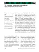
Figure 2: Plot of the density function of a Dirich-
let distribution H (the surface) as well as a draw
G (the vertical lines, or sticks) from a Dirichlet
process DP(α
0
, H) which has H as a base mea-
sure. Both distributions are defined over a sim-
plex in which each point corresponds to a particular
multinomial distribution over three possible words:
“profit”, “game”, and “election”. The placement of

the sticks is drawn from the distribution H, and is
independent of their lengths, which is drawn from a
stick-breaking process with parameter α
0
.
document by first generating a distribution over top-
ics π, and then for each position i in the document,
generating a topic z
i
from π, and then a word x
i
from the topic specific distribution φ
z
i
. The word
distributions φ
k
for each topic k are drawn from a
base distribution H. In Section 2, we sample C
multinomials φ
k
from H. In the infinite mixture
model we sample an infinite number of multinomi-
als from H, using the Dirichlet process.
Formally, given a base distribution H and a con-
centration parameter α
0
(loosely speaking, this con-
trols the relative sizes of the topics), a Dirichlet pro-
cess DP(α

0
, H) is the distribution of a discrete ran-
dom probability measure G over the same (possibly
continuous) space that H is defined over; thus it is a
measure over measures. In Figure 2, the sticks (ver-
tical lines) show a draw G from a Dirichlet process
where the base measure H is a Dirichlet distribution
over 3 words. A draw comprises of an infinite num-
ber of sticks, and each corresponding topic.
We factor G into two coindexed distributions: π,
a distribution over the integers, where the integer
represents the index of a particular topic (i.e., the
height of the sticks in the figure represent the proba-
bility of the topic indexed by that stick) and φ, rep-
resenting the word distribution of each of the top-
N
∞
α
0
H
π
φ
k
z
i
x
i
π|α
0
∼ GEM(α

0
)
φ
k
|H ∼ H
z
i
|π ∼ π
x
i
|z
i
, φ ∼ F (φ
z
i
)
N
∞
γ
α
0
β
H
π
j
φ
k
z
ji
x

ji
(a) (b)
Figure 3: A graphical representation of a simple
Dirichlet process mixture model (left) and a hierar-
chical Dirichlet process model (right). Note that we
show the stick-breaking representations of the mod-
els, in which we have factored G ∼ DP(α
0
, H) into
two sets of variables: π and φ.
ics (i.e., the location of the sticks in the figure). To
generate π we first generate an infinite sequence of
variables π
′
= (π
′
k
)
∞
k=1
, each of which is distributed
according to the Beta distribution:
π
′
k
|α
0
∼ Beta(1, α
0
)

Then π = (π
k
)
∞
k=1
is defined as:
π
k
= π
′
k

k−1
i=1
(1 − π
′
i
)
Following Pitman (2002) we refer to this process as
π ∼ GEM(α
0
). It should be noted that

∞
k=1
π
k
=
1,
5

and P (i) = π
i
. Then, according to the DP,
P (φ
i
) = π
i
. The complete model, is shown graphi-
cally in Figure 3(a).
To build intuition, we walk through the process of
generating from the infinite mixture model for the
document example, where x
i
is the word at posi-
tion i, and z
i
is its topic. F is a multinomial dis-
tribution parameterized by φ, and H is a Dirichlet
distribution. Instead of generating all of the infinite
mixture components (π
k
)
∞
k=1
at once, we can build
them up incrementally. If there are K known top-
ics, we represent only the known elements (π
k
)
K

k=1
and represent the remaining probability mass π
u
=
5
This is called the stick-breaking construction: we start with
a stick of unit length, representing the entire probability mass,
and successively break bits off the end of the stick, where the
proportional amount broken off is represented by π
′
k
and the
absolute amount is represented by π
k
.
274
φ
1
φ
2
φ
3
φ
4
φ
5
φ
6
φ
7

. . .
β :
π
j
:
. . .
Figure 4: A graphical representation of π
j
, a broken
stick, which is distributed according to a DP with a
broken stick β as a base measure. Each β
k
corre-
sponds to a φ
k
.
1 − (

K
k=1
π
k
). Initially we have π
u
= 1 and
φ = ().
For the ith position in the document, we first draw
a topic z
i
∼ π. If z

i
= u, then we find the coin-
dexed topic φ
z
i
. If z
i
= u, the unseen topic, we
make a draw b ∼ Beta(1, α
0
) and set π
K+1
= bπ
u
and π
new
u
= (1 − b)π
u
. Then we draw a parame-
ter φ
K+1
∼ H for the new topic, resulting in π =
(π
1
, . . . , π
K+1
, π
new
u

) and φ = (φ
1
, . . . , φ
K+1
). A
word is then drawn from this topic and emitted by
the document.
3.2 The Hierarchical Dirichlet Process
Let’s generalize our previous example to a corpus
of documents. As before, we have a set of shared
topics, but now each document has its own charac-
teristic distribution over these topics. We represent
topic distributions both locally (for each document)
and globally (across all documents) by use of a hier-
archical Dirichlet process (HDP), which has a local
DP for each document, in which the base measure is
itself a draw from another, global, DP.
The complete HDP model is represented graphi-
cally in Figure 3(b). Like the DP, it has global bro-
ken stick β = (β
k
)
∞
k=1
and topic specific word dis-
tribution parameters φ = (φ
k
)
∞
k=1

, which are coin-
dexed. It differs from the DP in that it also has lo-
cal broken sticks π
j
for each group j (in our case
documents). While the global stick β ∼ GEM(γ)
is generated as before, the local sticks π
j
are dis-
tributed according to a DP with base measure β:
π
j
∼ DP(α
0
, β).
We illustrate this generation process in Figure 4.
The upper unit line represents β, where the size of
segment k represents the value of element β
k
, and
the lower unit line represents π
j
∼ DP(α
0
, β) for a
particular group j. Each element of the lower stick
was sampled from a particular element of the upper
stick, and elements of the upper stick may be sam-
pled multiple times or not at all; on average, larger
elements will be sampled more often. Each element

β
k
, as well as all elements of π
j
that were sampled
from it, corresponds to a particular φ
k
. Critically,
several distinct π
j
can be sampled from the same
β
k
and hence share φ
k
; this is how components are
shared among groups.
For concreteness, we show how to generate a cor-
pus of documents from the HDP, generating one
document at a time, and incrementally construct-
ing our infinite objects. Initially we have β
u
= 1,
φ = (), and π
ju
= 1 for all j. We start with the
first position of the first document and draw a local
topic y
11
∼ π

1
, which will return u with probabil-
ity 1. Because y
11
= u we must make a draw from
the base measure, β, which, because this is the first
document, will also return u with probability 1. We
must now break β
u
into β
1
and β
new
u
, and break π
1u
into π
11
and π
new
1u
in the same manner presented for
the DP. Since π
11
now corresponds to global topic
1, we sample the word x
11
∼ Multinomial(φ
1
). To

sample each subsequent word i, we first sample the
local topic y
1i
∼ π
1
. If y
1i
= u, and π
1y
1i
corre-
sponds to β
k
in the global stick, then we sample the
word x
1i
∼ Multinomial(φ
k
). Once the first docu-
ment has been sampled, subsequent documents are
sampled in a similar manner; initially π
ju
= 1 for
document j, while β continues to grow as more doc-
uments are sampled.
4 Infinite Trees
We now use the techniques from Section 3 to create
infinite versions of each tree model from Section 2.
4.1 Independent Children
The changes required to make the Bayesian inde-

pendent children model infinite don’t affect its ba-
sic structure, as can be witnessed by comparing the
graphical depiction of the infinite model in Figure 5
with that of the finite model in Figure 1. The in-
stance variables z
t
and x
t
are parameterized as be-
fore. The primary change is that the number of
copies of the state plate is infinite, as are the number
of variables π
k
and φ
k
.
Note also that each distribution over possible
child states π
k
must also be infinite, since the num-
ber of possible child states is potentially infinite. We
achieve this by representing each of the π
k
variables
as a broken stick, and adopt the same approach of
275
β|γ ∼ GEM(γ)
π
k
|α

0
, β ∼ DP(α
0
, β)
φ
k
|H ∼ H
∞
γ
β
α
0
π
k
H
φ
k
z
1
z
2
z
3
x
1
x
2
x
3
Figure 5: A graphical representation of the infinite

independent child model.
sampling each π
k
from a DP with base measure β.
For the dependency tree application, φ
k
is a vector
representing the parameters of a multinomial over
words, and H is a Dirichlet distribution.
The infinite hidden Markov model (iHMM) or
HDP-HMM (Beal et al., 2002; Teh et al., 2006) is
a model of sequence data with transitions modeled
by an HDP.
6
The iHMM can be viewed as a special
case of this model, where each state (except the stop
state) produces exactly one child.
4.2 Simultaneous Children
The key problem in the definition of the simulta-
neous children model is that of defining a distribu-
tion over the lists of children produced by each state,
since each child in the list has as its domain the posi-
tive integers, representing the infinite set of possible
states. Our solution is to construct a distribution L
k
over lists of states from the distribution over individ-
ual states π
k
. The obvious approach is to sample the
states at each position i.i.d.:

P((z
t
′
)
t
′
∈c(t)
|π) =

t
′
∈c(t)
P(z
t
′
|π) =

t
′
∈c(t)
π
z
t
′
However, we want our model to be able to rep-
resent the fact that some child lists, c
t
, are more
or less probable than the product of the individual
child probabilities would indicate. To address this,

we can sample a state-conditional distribution over
child lists λ
k
from a DP with L
k
as a base measure.
6
The original iHMM paper (Beal et al., 2002) predates, and
was the motivation for, the work presented in Teh et al. (2006),
and is the origin of the term hierarchical Dirichlet process.
However, they used the term to mean something slightly differ-
ent than the HDP presented in Teh et al. (2006), and presented a
sampling scheme for inference that was a heuristic approxima-
tion of a Gibbs sampler.
Thus, we augment the basic model given in the pre-
vious section with the variables ζ, L
k
, and λ
k
:
L
k
|π
k
∼ Deterministic, as described above
λ
k
|ζ, L
k
∼ DP(ζ, L

k
)
c
t
|λ
k
∼ λ
k
An important consequence of defining L
k
locally
(instead of globally, using β instead of the π
k
s) is
that the model captures not only what sequences of
children a state prefers, but also the individual chil-
dren that state prefers; if a state gives high proba-
bility to some particular sequence of children, then
it is likely to also give high probability to other se-
quences containing those same states, or a subset
thereof.
4.3 Markov Children
In the Markov children model, more copies of the
variable π are needed, because each child state must
be conditioned both on the parent state and on the
state of the preceding child. We use a new set of
variables π
ki
, where π is determined by the par-
ent state k and the state of the preceding sibling i.

Each of the π
ki
is distributed as π
k
was in the basic
model: π
ki
∼ DP(α
0
, β).
5 Inference
Our goal in inference is to draw a sample from the
posterior over assignments of states to observations.
We present an inference procedure for the infinite
tree that is based on Gibbs sampling in the direct
assignment representation, so named because we di-
rectly assign global state indices to observations.
7
Before we present the procedure, we define a few
count variables. Recall from Figure 4 that each state
k has a local stick π
k
, each element of which cor-
responds to an element of β. In our sampling pro-
cedure, we only keep elements of π
k
and β which
correspond to states observed in the data. We define
the variable m
jk

to be the number of elements of the
finite observed portion of π
k
which correspond to β
j
and n
jk
to be the number of observations with state
k whose parent’s state is j.
We also need a few model-specific counts. For the
simultaneous children model we need
n
jz
, which is
7
We adapt one of the sampling schemes mentioned by Teh
et al. (2006) for use in the iHMM. This paper suggests two
sampling schemes for inference, but does not explicitly present
them. Upon discussion with one of the authors (Y. W. Teh,
2006, p.c.), it became clear that inference using the augmented
representation is much more complicated than initially thought.
276
the number of times the state sequence z occurred
as the children of state j. For the Markov chil-
dren model we need the count variable ˆn
jik
which
is the number of observations for a node with state
k whose parent’s state is j and whose previous sib-
ling’s state is i. In all cases we represent marginal

counts using dot-notation, e.g., n
·k
is the total num-
ber of nodes with state k, regardless of parent.
Our procedure alternates between three distinct
sampling stages: (1) sampling the state assignments
z, (2) sampling the counts m
jk
, and (3) sampling
the global stick β. The only modification of the pro-
cedure that is required for the different tree mod-
els is the method for computing the probability
of the child state sequence given the parent state
P((z
t
′
)
t
′
∈c(t)
|z
t
), defined separately for each model.
Sampling z. In this stage we sample a state for
each tree node. The probability of node t being as-
signed state k is given by:
P(z
t
= k|z
−t

, β) ∝ P(z
t
= k, (z
t
′
)
t
′
∈s(t)
|z
p(t)
)
· P((z
t
′
)
t
′
∈c(t)
|z
t
= k) · f
−x
t
k
(x
t
)
where s(t) denotes the set of siblings of t, f
−x

t
k
(x
t
)
denotes the posterior probability of observation x
t
given all other observations assigned to state k, and
z
−t
denotes all state assignments except z
t
. In other
words, the probability is proportional to the product
of three terms: the probability of the states of t and
its siblings given its parent z
p(t)
, the probability of
the states of the children c(t) given z
t
, and the pos-
terior probability of observation x
t
given z
t
. Note
that if we sample z
t
to be a previously unseen state,
we will need to extend β as discussed in Section 3.2.

Now we give the equations for P((z
t
′
)
t
′
∈c(t)
|z
t
)
for each of the models. In the independent child
model the probability of generating each child is:
P
ind
(z
c
i
(t)
= k|z
t
= j) =
n
jk
+ α
0
β
k
n
j·
+ α

0
P
ind
((z
t
′
)
t
′
∈c(t)
|z
t
= j) =

t
′
∈c(t)
P
ind
(z
t
′
|z
t
= j)
For the simultaneous child model, the probability of
generating a sequence of children, z, takes into ac-
count how many times that sequence has been gen-
erated, along with the likelihood of regenerating it:
P

sim
((z
t
′
)
t
′
∈c(t)
= z|z
t
= j) =
n
jz
+ ζP
ind
(z|z
t
= j)
n
j·
+ ζ
Recall that ζ denotes the concentration parameter
for the sequence generating DP. Lastly, we have the
DT NN IN DT NN VBD PRP$ NN TO VB NN EOS
The man in the corner taught his dachshund to play golf EOS
Figure 6: An example of a syntactic dependency tree
where the dependencies are between tags (hidden
states), and each tag generates a word (observation).
Markov child model:
P

m
(z
c
i
(t)
= k|z
c
i−1
(t)
= i, z
t
= j) =
ˆn
jik
+ α
0
β
k
ˆn
ji·
+ α
0
P
m
((z
t
′
)
t
′

∈c(t)
|z
t
) =

|c(t)|
i=1
P
m
(z
c
i
(t)
|z
c
i−1
(t)
, z
t
)
Finally, we give the posterior probability of an ob-
servation, given that F (φ
k
) is Multinomial(φ
k
), and
that H is Dirichlet(ρ, . . . , ρ). Let N be the vocab-
ulary size and ˙n
k
be the number of observations x

with state k. Then:
f
−x
t
k
(x
t
) =
˙n
x
t
k
+ ρ
˙n
·k
+ N ρ
Sampling m. We use the following procedure,
which slightly modifies one from (Y. W. Teh, 2006,
p.c.), to sample each m
jk
:
SAMPLEM(j, k)
1 if n
jk
= 0
2 then m
jk
= 0
3 else m
jk

= 1
4 for i ← 2 to n
jk
5 do if rand() <
α
0
α
0
+i−1
6 then m
jk
= m
jk
+ 1
7 return m
jk
Sampling β. Lastly, we sample β using the Di-
richlet distribution:
(β
1
, . . . , β
K
, β
u
) ∼ Dirichlet(m
·1
, . . . , m
·K
, α
0

)
6 Experiments
We demonstrate infinite tree models on two dis-
tinct syntax learning tasks: unsupervised POS learn-
ing conditioned on untagged dependency trees and
learning a split of an existing tagset, which improves
the accuracy of an automatic syntactic parser.
For both tasks, we use a simple modification of
the basic model structure, to allow the trees to gen-
erate dependents on the left and the right with dif-
ferent distributions – as is useful in modeling natu-
ral language. The modification of the independent
child tree is trivial: we have two copies of each of
277
the variables π
k
, one each for the left and the right.
Generation of dependents on the right is completely
independent of that for the left. The modifications of
the other models are similar, but now there are sepa-
rate sets of π
k
variables for the Markov child model,
and separate L
k
and λ
k
variables for the simultane-
ous child model, for each of the left and right.
For both experiments, we used dependency trees

extracted from the Penn Treebank (Marcus et al.,
1993) using the head rules and dependency extrac-
tor from Yamada and Matsumoto (2003). As is stan-
dard, we used WSJ sections 2–21 for training, sec-
tion 22 for development, and section 23 for testing.
6.1 Unsupervised POS Learning
In the first experiment, we do unsupervised part-of-
speech learning conditioned on dependency trees.
To be clear, the input to our algorithm is the de-
pendency structure skeleton of the corpus, but not
the POS tags, and the output is a labeling of each
of the words in the tree for word class. Since the
model knows nothing about the POS annotation, the
new classes have arbitrary integer names, and are
not guaranteed to correlate with the POS tag def-
initions. We found that the choice of α
0
and β
(the concentration parameters) did not affect the out-
put much, while the value of ρ (the parameter for
the base Dirichlet distribution) made a much larger
difference. For all reported experiments, we set
α
0
= β = 10 and varied ρ.
We use several metrics to evaluate the word
classes. First, we use the standard approach of
greedily assigning each of the learned classes to the
POS tag with which it has the greatest overlap, and
then computing tagging accuracy (Smith and Eisner,

2005; Haghighi and Klein, 2006).
8
Additionally, we
compute the mutual information of the learned clus-
ters with the gold tags, and we compute the cluster
F-score (Ghosh, 2003). See Table 1 for results of
the different models, parameter settings, and met-
rics. Given the variance in the number of classes
learned it is a little difficult to interpret these results,
but it is clear that the Markov child model is the
best; it achieves superior performance to the inde-
pendent child model on all metrics, while learning
fewer word classes. The poor performance of the
simultaneous model warrants further investigation,
but we observed that the distributions learned by that
8
The advantage of this metric is that it’s comprehensible.
The disadvantage is that it’s easy to inflate by adding classes.
Model ρ # Classes Acc. MI F1
Indep. 0.01 943 67.89 2.00 48.29
0.001 1744 73.61 2.23 40.80
0.0001 2437 74.64 2.27 39.47
Simul. 0.01 183 21.36 0.31 21.57
0.001 430 15.77 0.09 13.80
0.0001 549 16.68 0.12 14.29
Markov 0.01 613 68.53 2.12 49.82
0.001 894 75.34 2.31 48.73
Table 1: Results of part unsupervised POS tagging
on the different models, using a greedy accuracy
measure.

model are far more spiked, potentially due to double
counting of tags, since the sequence probabilities are
already based on the local probabilities.
For comparison, Haghighi and Klein (2006) re-
port an unsupervised baseline of 41.3%, and a best
result of 80.5% from using hand-labeled prototypes
and distributional similarity. However, they train on
less data, and learn fewer word classes.
6.2 Unsupervised POS Splitting
In the second experiment we use the infinite tree
models to learn a refinement of the PTB tags. We
initialize the set of hidden states to the set of PTB
tags, and then, during inference, constrain the sam-
pling distribution over hidden state z
t
at each node t
to include only states that are a refinement of the an-
notated PTB tag at that position. The output of this
training procedure is a new annotation of the words
in the PTB with the learned tags. We then compare
the performance of a generative dependency parser
trained on the new refined tags with one trained on
the base PTB tag set. We use the generative de-
pendency parser distributed with the Stanford fac-
tored parser (Klein and Manning, 2003b) for the
comparison, since it performs simultaneous tagging
and parsing during testing. In this experiment, un-
labeled, directed, dependency parsing accuracy for
the best model increased from 85.11% to 87.35%, a
15% error reduction. See Table 2 for the full results

over all models and parameter settings.
7 Related Work
The HDP-PCFG (Liang et al., 2007), developed at
the same time as this work, aims to learn state splits
for a binary-branching PCFG. It is similar to our
simultaneous child model, but with several impor-
tant distinctions. As discussed in Section 4.2, in our
model each state has a DP over sequences, with a
base distribution that is defined over the local child
278
Model ρ Accuracy
Baseline – 85.11
Independent 0.01 86.18
0.001 85.88
Markov 0.01 87.15
0.001 87.35
Table 2: Results of untyped, directed dependency
parsing, where the POS tags in the training data have
been split according to the various models. At test
time, the POS tagging and parsing are done simulta-
neously by the parser.
state probabilities. In contrast, Liang et al. (2007)
define a global DP over sequences, with the base
measure defined over the global state probabilities,
β; locally, each state has an HDP, with this global
DP as the base measure. We believe our choice to
be more linguistically sensible: in our model, for a
particular state, dependent sequences which are sim-
ilar to one another increase one another’s likelihood.
Additionally, their modeling decision made it diffi-

cult to define a Gibbs sampler, and instead they use
variational inference. Earlier, Johnson et al. (2007)
presented adaptor grammars, which is a very simi-
lar model to the HDP-PCFG. However they did not
confine themselves to a binary branching structure
and presented a more general framework for defin-
ing the process for splitting the states.
8 Discussion and Future Work
We have presented a set of novel infinite tree models
and associated inference algorithms, which are suit-
able for representing syntactic dependency structure.
Because the models represent a potentially infinite
number of hidden states, they permit unsupervised
learning algorithms which naturally select a num-
ber of word classes, or tags, based on qualities of
the data. Although they require substantial techni-
cal background to develop, the learning algorithms
based on the models are actually simple in form, re-
quiring only the maintenance of counts, and the con-
struction of sampling distributions based on these
counts. Our experimental results are preliminary but
promising: they demonstrate that the model is capa-
ble of capturing important syntactic structure.
Much remains to be done in applying infinite
models to language structure, and an interesting ex-
tension would be to develop inference algorithms
that permit completely unsupervised learning of de-
pendency structure.
Acknowledgments
Many thanks to Yeh Whye Teh for several enlight-

ening conversations, and to the following mem-
bers (and honorary member) of the Stanford NLP
group for comments on an earlier draft: Thad
Hughes, David Hall, Surabhi Gupta, Ani Nenkova,
Sebastian Riedel. This work was supported by a
Scottish Enterprise Edinburgh-Stanford Link grant
(R37588), as part of the EASIE project, and by
the Advanced Research and Development Activity
(ARDA)’s Advanced Question Answering for Intel-
ligence (AQUAINT) Phase II Program.
References
C. E. Antoniak. 1974. Mixtures of Dirichlet processes with ap-
plications to Bayesian nonparametrics. Annals of Statistics,
2:1152–1174.
M.J. Beal, Z. Ghahramani, and C.E. Rasmussen. 2002. The
infinite hidden Markov model. In Advances in Neural Infor-
mation Processing Systems, pages 577–584.
E. Charniak. 1996. Tree-bank grammars. In AAAI 1996, pages
1031–1036.
E. Charniak. 2000. A maximum-entropy-inspired parser. In
HLT-NAACL 2000, pages 132–139.
M. Collins. 2003. Head-driven statistical models for natural lan-
guage parsing. Computational Linguistics, 29(4):589–637.
T. S. Ferguson. 1973. A Bayesian analysis of some nonpara-
metric problems. Annals of Statistics, 1:209–230.
J. Ghosh. 2003. Scalable clustering methods for data mining. In
N. Ye, editor, Handbook of Data Mining, chapter 10, pages
247–277. Lawrence Erlbaum Assoc.
A. Haghighi and D. Klein. 2006. Prototype-driven learning for
sequence models. In HLT-NAACL 2006.

M. Johnson, T. Griffiths, and S. Goldwater. 2007. Adaptor
grammars: A framework for specifying compositional non-
parametric Bayesian models. In NIPS 2007.
D. Klein and C. D. Manning. 2003a. Accurate unlexicalized
parsing. In ACL 2003.
D. Klein and C. D. Manning. 2003b. Factored A* search for
models over sequences and trees. In IJCAI 2003.
P. Liang, S. Petrov, D. Klein, and M. Jordan. 2007. Nonpara-
metric PCFGs using Dirichlet processes. In EMNLP 2007.
M. P. Marcus, B. Santorini, and M. A. Marcinkiewicz. 1993.
Building a large annotated corpus of English: The Penn
Treebank. Computational Linguistics, 19(2):313–330.
S. Petrov, L. Barrett, R. Thibaux, and D. Klein. 2006. Learning
accurate, compact, and interpretable tree annotation. In ACL
44/COLING 21, pages 433–440.
J. Pitman. 2002. Poisson-Dirichlet and GEM invariant distribu-
tions for split-and-merge transformations of an interval par-
tition. Combinatorics, Probability and Computing, 11:501–
514.
N. A. Smith and J. Eisner. 2005. Contrastive estimation: Train-
ing log-linear models on unlabeled data. In ACL 2005.
Y. W. Teh, M.I. Jordan, M. J. Beal, and D.M. Blei. 2006. Hier-
archical Dirichlet processes. Journal of the American Statis-
tical Association, 101:1566–1581.
H. Yamada and Y. Matsumoto. 2003. Statistical dependency
analysis with support vector machines. In Proceedings of
IWPT, pages 195–206.
279