Báo cáo khoa học: "A Geometric View on Bilingual Lexicon Extraction from Comparable Corpora" pptx
Bạn đang xem bản rút gọn của tài liệu. Xem và tải ngay bản đầy đủ của tài liệu tại đây (114.34 KB, 8 trang )
A Geometric View on Bilingual Lexicon Extraction from Comparable
Corpora
E. Gaussier
†
, J M. Renders
†
, I. Matveeva
∗
, C. Goutte
†
, H. D
´
ejean
†
†
Xerox Research Centre Europe
6, Chemin de Maupertuis — 38320 Meylan, France
∗
Dept of Computer Science, University of Chicago
1100 E. 58th St. Chicago, IL 60637 USA
Abstract
We present a geometric view on bilingual lexicon
extraction from comparable corpora, which allows
to re-interpret the methods proposed so far and iden-
tify unresolved problems. This motivates three new
methods that aim at solving these problems. Empir-
ical evaluation shows the strengths and weaknesses
of these methods, as well as a significant gain in the
accuracy of extracted lexicons.
1 Introduction
Comparable corpora contain texts written in differ-
ent languages that, roughly speaking, ”talk about
the same thing”. In comparison to parallel corpora,
ie corpora which are mutual translations, compara-
ble corpora have not received much attention from
the research community, and very few methods have
been proposed to extract bilingual lexicons from
such corpora. However, except for those found in
translation services or in a few international organ-
isations, which, by essence, produce parallel docu-
mentations, most existing multilingual corpora are
not parallel, but comparable. This concern is re-
flected in major evaluation conferences on cross-
language information retrieval (CLIR), e.g. CLEF
1
,
which only use comparable corpora for their multi-
lingual tracks.
We adopt here a geometric view on bilingual lex-
icon extraction from comparable corpora which al-
lows one to re-interpret the methods proposed thus
far and formulate new ones inspired by latent se-
mantic analysis (LSA), which was developed within
the information retrieval (IR) community to treat
synonymous and polysemous terms (Deerwester et
al., 1990). We will explain in this paper the moti-
vations behind the use of such methods for bilin-
gual lexicon extraction from comparable corpora,
and show how to apply them. Section 2 is devoted to
the presentation of the standard approach, ie the ap-
proach adopted by most researchers so far, its geo-
metric interpretation, and the unresolved synonymy
1
:2002/
and polysemy problems. Sections 3 to 4 then de-
scribe three new methods aiming at addressing the
issues raised by synonymy and polysemy: in sec-
tion 3 we introduce an extension of the standard ap-
proach, and show in appendix A how this approach
relates to the probabilistic method proposed in (De-
jean et al., 2002); in section 4, we present a bilin-
gual extension to LSA, namely canonical correla-
tion analysis and its kernel version; lastly, in sec-
tion 5, we formulate the problem in terms of prob-
abilistic LSA and review different associated simi-
larities. Section 6 is then devoted to a large-scale
evaluation of the different methods proposed. Open
issues are then discussed in section 7.
2 Standard approach
Bilingual lexicon extraction from comparable cor-
pora has been studied by a number of researchers,
(Rapp, 1995; Peters and Picchi, 1995; Tanaka and
Iwasaki, 1996; Shahzad et al., 1999; Fung, 2000,
among others). Their work relies on the assump-
tion that if two words are mutual translations, then
their more frequent collocates (taken here in a very
broad sense) are likely to be mutual translations as
well. Based on this assumption, the standard ap-
proach builds context vectors for each source and
target word, translates the target context vectors us-
ing a general bilingual dictionary, and compares the
translation with the source context vector:
1. For each source word v (resp. target word w),
build a context vector
−→
v (resp.
−→
w ) consisting
in the measure of association of each word e
(resp. f) in the context of v (resp. w), a(v, e).
2. Translate the context vectors with a general
bilingual dictionary D, accumulating the con-
tributions from words that yield identical trans-
lations.
3. Compute the similarity between source word v
and target word w using a similarity measures,
such as the Dice or Jaccard coefficients, or the
cosine measure.
As the dot-product plays a central role in all these
measures, we consider, without loss of generality,
the similarity given by the dot-product between
−→
v
and the translation of
−→
w :
−→
v ,
−−−→
tr(w) =
e
a(v, e)
f,(e,f )inD
a(w, f)
=
(e,f)∈D
a(v, e) a(w, f) (1)
Because of the translation step, only the pairs (e, f)
that are present in the dictionary contribute to the
dot-product.
Note that this approach requires some general
bilingual dictionary as initial seed. One way to cir-
cumvent this requirement consists in automatically
building a seed lexicon based on spelling and cog-
nates clues (Koehn and Knight, 2002). Another ap-
proach directly tackles the problem from scratch by
searching for a translation mapping which optimally
preserves the intralingual association measure be-
tween words (Diab and Finch, 2000): the under-
lying assumption is that pairs of words which are
highly associated in one languageshouldhave trans-
lations that are highly associated in the other lan-
guage. In this latter case, the association measure
is defined as the Spearman rank order correlation
between their context vectors restricted to “periph-
eral tokens” (highly frequent words). The search
method is based on a gradient descent algorithm, by
iteratively changing the mapping of a single word
until (locally) minimizing the sum of squared differ-
ences between the association measure of all pairs
of words in one language and the association mea-
sure of the pairs of translated words obtained by the
current mapping.
2.1 Geometric presentation
We denote by s
i
, 1 ≤ i ≤ p and t
j
, 1 ≤ j ≤ q the
source and target words in the bilingual dictionary
D. D is a set of n translation pairs (s
i
, t
j
), and
may be represented as a p × q matrix M, such that
M
ij
= 1 iff (s
i
, t
j
) ∈ D (and 0 otherwise).
2
Assuming there are m distinct source words
e
1
, · · · , e
m
and r distinct target words f
1
, · · · , f
r
in
the corpus, figure 1 illustrates the geometric view of
the standard method.
The association measure a(v, e) may be viewed
as the coordinates of the m-dimensional context
vector
−→
v in the vector space formed by the or-
thogonal basis (e
1
, · · · , e
m
). The dot-product in (1)
only involves source dictionary entries. The corre-
sponding dimensions are selected by an orthogonal
2
The extension to weighted dictionary entries M
ij
∈ [0, 1]
is straightforward but not considered here for clarity.
projection on the sub-space formed by (s
1
, · · · , s
p
),
using a p × m projection matrix P
s
. Note that
(s
1
, · · · , s
p
), being a sub-family of (e
1
, · · · , e
m
), is
an orthogonal basis of the new sub-space. Similarly,
−→
w is projected on the dictionary entries (t
1
, · · · , t
q
)
using a q × r orthogonal projection matrix P
t
. As
M encodes the relationship between the source and
target entries of the dictionary, equation 1 may be
rewritten as:
S(v, w) =
−→
v ,
−−−→
tr(w) = (P
s
−→
v )
M (P
t
−→
w ) (2)
where
denotes transpose. In addition, notice that
M can be rewritten as S
T , with S an n × p and
T an n × q matrix encoding the relations between
words and pairs in the bilingual dictionary (e.g. S
ki
is 1 iff s
i
is in the k
th
translation pair). Hence:
S(v, w)=
−→
v
P
s
S
T P
t
−→
w =SP
s
−→
v , T P
t
−→
w (3)
which shows that the standard approach amounts to
performing a dot-product in the vector space formed
by the n pairs ((s
1
, t
l
), · · · , (s
p
, t
k
)), which are as-
sumed to be orthogonal, and correspond to transla-
tion pairs.
2.2 Problems with the standard approach
There are two main potential problems associated
with the use of a bilingual dictionary.
Coverage. This is a problem if too few corpus
words are covered by the dictionary. However, if
the context is large enough, some context words
are bound to belong to the general language, so a
general bilingual dictionary should be suitable. We
thus expect the standard approach to cope well with
the coverage problem, at least for frequent words.
For rarer words, we can bootstrap the bilingual dic-
tionary by iteratively augmenting it with the most
probable translations found in the corpus.
Polysemy/synonymy. Because all entries on ei-
ther side of the bilingual dictionary are treated as or-
thogonal dimensions in the standard methods, prob-
lems may arise when several entries have the same
meaning (synonymy), or when an entry has sev-
eral meanings (polysemy), especially when only
one meaning is represented in the corpus.
Ideally, the similarities wrt synonyms should not
be independent, but the standard method fails to ac-
count for that. The axes corresponding to synonyms
s
i
and s
j
are orthogonal, so that projections of a
context vector on s
i
and s
j
will in general be uncor-
related. Therefore, a context vector that is similar to
s
i
may not necessarily be similar to s
j
.
A similar situation arises for polysemous entries.
Suppose the word bank appears as both financial in-
stitution (French: banque) and ground near a river
P
s
e
2
e
m
v
e
1
s
1
s
p
v’
(s ,t )
t
t
f
f
f(s ,t )
1 1
(s ,t )
2
1
r
w
w’
1
p
P
t
S T
p k
1 i
v"
w"
Figure 1: Geometric view of the standard approach
(French: berge), but only the pair (banque, bank)
is in the bilingual dictionary. The standard method
will deem similar river, which co-occurs with bank,
and argent (money), which co-occurs with banque.
In both situations, however, the context vectors of
the dictionary entries provide some additional infor-
mation: for synonyms s
i
and s
j
, it is likely that
−→
s
i
and
−→
s
j
are similar; for polysemy, if the context vec-
tors
−−−−→
banque and
−−→
bank have few translations pairs in
common, it is likely that banque and bank are used
with somewhat different meanings. The following
methods try to leverage this additional information.
3 Extension of the standard approach
The fact that synonyms may be captured through
similarity of context vectors
3
leads us to question
the projection that is made in the standard method,
and to replace it with a mapping into the sub-space
formed by the context vectors of the dictionary en-
tries, that is, instead of projecting
−→
v on the sub-
space formed by (s
1
, · · · , s
p
), we now map it onto
the sub-space generated by (
−→
s
1
, · · · ,
−→
s
p
). With this
mapping, we try to find a vector space in which syn-
onymous dictionary entries are close to each other,
while polysemous ones still select different neigh-
bors. This time, if
−→
v is close to
−→
s
i
and
−→
s
j
, s
i
and
s
j
being synonyms, the translations of both s
i
and
s
j
will be used to find those words w close to v.
Figure 2 illustrates this process. By denoting Q
s
,
respectively Q
t
, such a mapping in the source (resp.
target) side, and using the same translation mapping
(S, T ) as above, the similarity between source and
target words becomes:
S(v, w)=SQ
s
−→
v , T Q
t
−→
w =
−→
v
Q
s
S
T Q
t
−→
w (4)
A natural choice for Q
s
(and similarly for Q
t
) is the
following m × p matrix:
Q
s
= R
s
=
a(s
1
, e
1
) · · · a(s
p
, e
1
)
.
.
.
.
.
.
.
.
.
a(s
1
, e
m
) · · · a(s
p
, e
m
)
3
This assumption has been experimentally validated in sev-
eral studies, e.g. (Grefenstette, 1994; Lewis et al., 1967).
but other choices, such as a pseudo-inverse of R
s
,
are possible. Note however that computing the
pseudo-inverse of R
s
is a complex operation, while
the above projection is straightforward (the columns
of Q correspond to the context vectors of the dic-
tionary words). In appendix A we show how this
method generalizes over the probabilistic approach
presented in (Dejean et al., 2002). The above
method bears similarities with the one described
in (Besanc¸on et al., 1999), where a matrix similar
to Q
s
is used to build a new term-document ma-
trix. However, the motivations behind their work
and ours differ, as do the derivations and the gen-
eral framework, which justifies e.g. the choice of
the pseudo-inverse of R
s
in our case.
4 Canonical correlation analysis
The data we have at our disposal can naturally be
represented as an n × (m + r) matrix in which
the rows correspond to translation pairs, and the
columns to source and target vocabularies:
C =
e
1
· · · e
m
f
1
· · · f
r
· · · · · · · · · · · · · · · · · · (s
(1)
, t
(1)
)
.
.
.
.
.
.
.
.
.
.
.
.
.
.
.
.
.
.
.
.
.
· · · · · · · · · · · · · · · · · · (s
(n)
, t
(n)
)
where (s
(k)
, t
(k)
) is just a renumbering of the trans-
lation pairs (s
i
, t
j
).
Matrix C shows that each translation pair sup-
ports two views, provided by the context vectors in
the source and target languages. Each view is con-
nected to the other by the translation pair it repre-
sents. The statistical technique of canonical corre-
lation analysis (CCA) can be used to identify direc-
tions in the source view (first m columns of C) and
target view (last r columns of C) that are maximally
correlated, ie “behave in the same way” wrt the
translation pairs. We are thus looking for directions
in the source and target vector spaces (defined by
the orthogonal bases (e
1
, · · · , e
m
) and (f
1
, · · · , f
r
))
such that the projections of the translation pairs on
these directions are maximally correlated. Intu-
itively, those directions define latent semantic axes
s
e
e
e
v
f
f
f(s ,t )
1
2
1
r
w
1
t
S T
e
m
e
1
e
2
m
1
2
s
s
s
s
(s ,t )
1
(s ,t )
p
1
k
i
f
f
r
2
f t
t
t
t
1
2
w"
v"
1
2
p
k
q
i
v
wQ Q
Figure 2: Geometric view of the extended approach
that capture the implicit relations between transla-
tion pairs, and induce a natural mapping across lan-
guages. Denoting by ξ
s
and ξ
t
the directions in the
source and target spaces, respectively, this may be
formulated as:
ρ = max
ξ
s
,ξ
t
i
ξ
s
,
−→
s
(i)
ξ
t
,
−→
t
(i)
i
ξ
s
,
−→
s
(i)
j
ξ
t
,
−→
t
(j)
As in principal component analysis, once the first
two directions (ξ
1
s
, ξ
1
t
) have been identified, the pro-
cess can be repeated in the sub-space orthogonal
to the one formed by the already identified direc-
tions. However, a general solution based on a set of
eigenvalues can be proposed. Following e.g. (Bach
and Jordan, 2001), the above problem can be re-
formulated as the following generalized eigenvalue
problem:
B ξ = ρD ξ (5)
where, denoting again R
s
and R
t
the first m and last
r (respectively) columns of C, we define:
B =
0 R
t
R
t
R
s
R
s
R
s
R
s
R
t
R
t
0
,
D =
(R
s
R
s
)
2
0
0 (R
t
R
t
)
2
, ξ =
ξ
s
ξ
t
The standard approach to solve eq. 5 is to per-
form an incomplete Cholesky decomposition of a
regularized form of D (Bach and Jordan, 2001).
This yields pairs of source and target directions
(ξ
1
s
, ξ
1
t
), · · · , (ξ
l
s
, ξ
l
t
) that define a new sub-space in
which to project words from each language. This
sub-space plays the same role as the sub-space de-
fined by translation pairs in the standard method, al-
though with CCA, it is derived from the corpus via
the context vectors of the translation pairs. Once
projected, words from different languages can be
compared through their dot-product or cosine. De-
noting Ξ
s
=
ξ
1
s
, . . . ξ
l
s
, and Ξ
t
=
ξ
1
t
, . . . ξ
l
t
,
the similarity becomes (figure 3):
S(v, w) = Ξ
s
−→
v , Ξ
t
−→
w =
−→
v
Ξ
s
Ξ
t
−→
w (6)
The number l of vectors retained in each language
directly defines the dimensions of the final sub-
space used for comparing words across languages.
CCA and its kernelised version were used in (Vi-
nokourov et al., 2002) as a way to build a cross-
lingual information retrieval system from parallel
corpora. We show here that it can be used to in-
fer language-independent semantic representations
from comparable corpora, which induce a similarity
between words in the source and target languages.
5 Multilingual probabilistic latent
semantic analysis
The matrix C described above encodes in each row
k the context vectors of the source (first m columns)
and target (last r columns) of each translation pair.
Ideally, we would like to cluster this matrix such
that translation pairs with synonymous words ap-
pear in the same cluster, while translation pairs with
polysemous words appear in different clusters (soft
clustering). Furthermore, because of the symmetry
between the roles played by translation pairs and vo-
cabulary words (synonymous and polysemous vo-
cabulary words should also behave as described
above), we want the clustering to behave symmet-
rically with respect to translation pairs and vocabu-
lary words. One well-motivated method that fulfills
all the above criteria is Probabilistic Latent Seman-
tic Analysis (PLSA) (Hofmann, 1999).
Assuming that C encodes the co-occurrences be-
tween vocabulary words w and translation pairs d,
PLSA models the probability of co-occurrence w
and d via latent classes α:
P (w, d) =
α
P (α) P (w|α) P (d|α) (7)
where, for a given class, words and translation pairs
are assumed to be independently generated from
class-conditional probabilities P (w|α) and P (d|α).
Note here that the latter distribution is language-
independent, and that the same latent classes are
used for the two languages. The parameters of the
model are obtained by maximizing the likelihood of
the observed data (matrix C) through Expectation-
Maximisation algorithm (Dempster et al., 1977). In
e
e
e
v
f
f
f
2
1
r
w
1
e
e
1
e
2
m
1
2
f
f
r
2
f
v"
v
w(CCA)
w"
(CCA)
m
(ξ
1
s
, ξ
1
t
)
ξ
1
s
ξ
i
s
ξ
l
s
ξ
2
s
(ξ
l
s
, ξ
l
t
)
(ξ
2
s
, ξ
2
t
) ξ
1
t
ξ
l
t
ξ
s
ξ
t
ξ
2
t
ξ
i
t
Figure 3: Geometric view of the Canonical Correlation Analysis approach
addition, in order to reduce the sensitivity to initial
conditions, we use a deterministic annealing scheme
(Ueda and Nakano, 1995). The update formulas for
the EM algorithm are given in appendix B.
This model can identify relevant bilingual latent
classes, but does not directly define a similarity be-
tween words across languages. That may be done
by using Fisher kernels as described below.
Associated similarities: Fisher kernels
Fisher kernels (Jaakkola and Haussler, 1999) de-
rive a similarity measure from a probabilistic model.
They are useful whenever a direct similarity be-
tween observed feature is hard to define or in-
sufficient. Denoting (w) = lnP(w|θ) the log-
likelihood for example w, the Fisher kernel is:
K(w
1
, w
2
) = ∇(w
1
)
I
F
−1
∇(w
2
) (8)
The Fisher information matrix I
F
=
E
∇(x)∇(x)
keeps the kernel indepen-
dent of reparameterisation. With a suitable
parameterisation, we assume I
F
≈ 1. For PLSA
(Hofmann, 2000), the Fisher kernel between two
words w
1
and w
2
becomes:
K(w
1
, w
2
) =
α
P (α|w
1
)P (α|w
2
)
P (α)
(9)
+
d
P (d|w
1
)
P (d|w
2
)
α
P (α|d,w
1
)P (α|d,w
2
)
P (d|α)
where d ranges over the translation pairs. The
Fisher kernel performs a dot-product in a vector
space defined by the parameters of the model. With
only one class, the expression of the Fisher kernel
(9) reduces to:
K(w
1
, w
2
) = 1 +
d
P (d|w
1
)
P (d|w
2
)
P (d)
Apart from the additional intercept (’1’), this is
exactly the similarity provided by the standard
method, with associations given by scaled empir-
ical frequencies a(w, d) =
P (d|w)/
P (d). Ac-
cordingly, we expect that the standard method and
the Fisher kernel with one class should have simi-
lar behaviors. In addition to the above kernel, we
consider two additional versions, obtained:through
normalisation (NFK) and exponentiation (EFK):
NF K(w
1
, w
2
) =
K(w
1
, w
2
)
K(w
1
)K(w
2
)
(10)
EFK(w
1
, w
2
) = e
−
1
2
(K(w
1
)+K(w
2
)−2K(w
1
,w
2
))
where K(w) stands for K(w, w).
6 Experiments and results
We conducted experiments on an English-French
corpus derived from the data used in the multi-
lingual track of CLEF2003, corresponding to the
newswire of months May 1994 and December 1994
of the Los Angeles Times (1994, English) and Le
Monde (1994, French). As our bilingual dictionary,
we used the ELRA multilingual dictionary,
4
which
contains ca. 13,500 entries with at least one match
in our corpus. In addition, the following linguis-
tic preprocessing steps were performed on both the
corpus and the dictionary: tokenisation, lemmatisa-
tion and POS-tagging. Only lexical words (nouns,
verbs, adverbs, adjectives) were indexed and only
single word entries in the dicitonary were retained.
Infrequent words (occurring less than 5 times) were
discarded when building the indexing terms and the
dictionary entries. After these steps our corpus con-
tains 34,966 distinct English words, and 21,140 dis-
tinct French words, leading to ca. 25,000 English
and 13,000 French words not present in the dictio-
nary.
To evaluate the performance of our extraction
methods, we randomly split the dictionaries into a
training set with 12,255 entries, and a test set with
1,245 entries. The split is designed in such a way
that all pairs corresponding to the same source word
are in the same set (training or test). All methods
use the training set as the sole available resource
and predict the most likely translations of the terms
in the source language (English) belonging to the
4
Available through www.elra.info
test set. The context vectors were defined by com-
puting the mutual information association measure
between terms occurring in the same context win-
dow of size 5 (ie. by considering a neighborhood of
+/- 2 words around the current word), and summing
it over all contexts of the corpora. Different associ-
ation measures and context sizes were assessed and
the above settings turned out to give the best perfor-
mance even if the optimum is relatively flat. For
memory space and computational efficiency rea-
sons, context vectors were pruned so that, for each
term, the remaining components represented at least
90 percent of the total mutual information. After
pruning, the context vectors were normalised so that
their Euclidean norm is equal to 1. The PLSA-based
methods used the raw co-occurrence counts as asso-
ciation measure, to be consistent with the underly-
ing generative model. In addition, for the extended
method, we retained only the N (N = 200 is the
value which yielded the best results in our experi-
ments) dictionary entries closest to source and tar-
get words when doing the projection with Q. As
discussed below, this allows us to get rid of spuri-
ous relationships.
The upper part of table 1 summarizes the results
we obtained, measured in terms of F-1 score for
different lengths of the candidate list, from 20 to
500. For each length, precision is based on the num-
ber of lists that contain an actual translation of the
source word, whereas recall is based on the num-
ber of translations provided in the reference set and
found in the list. Note that our results differ from the
ones previously published, which can be explained
by the fact that first our corpus is relatively small
compared to others, second that our evaluation re-
lies on a large number of candidates, which can oc-
cur as few as 5 times in the corpus, whereas previous
evaluations were based on few, high frequent terms,
and third that we do not use the same bilingual dic-
tionary, the coverage of which being an important
factor in the quality of the results obtained. Long
candidate lists are justified by CLIR considerations,
where longer lists might be preferred over shorter
ones for query expansion purposes. For PLSA, the
normalised Fisher kernels provided the best results,
and increasing the number of latent classes did not
lead in our case to improved results. We thus dis-
play here the results obtained with the normalised
version of the Fisher kernel, using only one compo-
nent. For CCA, we empirically optimised the num-
ber of dimensions to be used, and display the results
obtained with the optimal value (l = 300).
As one can note, the extended approach yields
the best results in terms of F1-score. However, its
performance for the first 20 candidates are below
the standard approach and comparable to the PLSA-
based method. Indeed, the standard approach leads
to higher precision at the top of the list, but lower
recall overall. This suggests that we could gain in
performance by re-ranking the candidates of the ex-
tended approach with the standard and PLSA meth-
ods. The lower part of table 1 shows that this is
indeed the case. The average precision goes up
from 0.4 to 0.44 through this combination, and the
F1-score is significantly improved for all the length
ranges we considered (bold line in table 1).
7 Discussion
Extended method As one could expect, the ex-
tended approach improves the recall of our bilingual
lexicon extraction system. Contrary to the standard
approach, in the extended approach, all the dictio-
nary words, present or not in the context vector of a
given word, can be used to translate it. This leads to
a noise problem since spurious relations are bound
to be detected. The restriction we impose on the
translation pairs to be used (N nearest neighbors)
directly aims at selecting only the translation pairs
which are in true relation with the word to be trans-
lated.
Multilingual PLSA Even though theoretically
well-founded, PLSA does not lead to improved per-
formance. When used alone, it performs slightly
below the standard method, for different numbers
of components, and performs similarly to the stan-
dard method when used in combination with the
extended method. We believe the use of mere co-
occurrence counts gives a disadvantage to PLSA
over other methods, which can rely on more sophis-
ticated measures. Furthermore, the complexity of
the final vector space (several millions of dimen-
sions) in which the comparison is done entails a
longer processing time, which renders this method
less attractive than the standard or extended ones.
Canonical correlation analysis The results we ob-
tain with CCA and its kernel version are disappoint-
ing. As already noted, CCA does not directly solve
the problems we mentioned, and our results show
that CCA does not provide a good alternative to the
standard method. Here again, we may suffer from a
noise problem, since each canonical direction is de-
fined by a linear combination that can involve many
different vocabulary words.
Overall, starting with an average precision of 0.35
as provided by the standard approach, we were able
to increase it to 0.44 with the methods we consider.
Furthermore, we have shown here that such an im-
provement could be achieved with relatively simple
20 60 100 160 200 260 300 400 500 Avg. Prec.
standard 0.14 0.20 0.24 0.29 0.30 0.33 0.35 0.38 0.40 0.35
Ext (N=500) 0.11 0.21 0.27 0.32 0.34 0.38 0.41 0.45 0.50 0.40
CCA (l=300) 0.04 0.10 0.14 0.20 0.22 0.26 0.29 0.35 0.41 0.25
NFK(k=1) 0.10 0.15 0.20 0.23 0.26 0.27 0.28 0.32 0.34 0.30
Ext + standard 0.16 0.26 0.32 0.37 0.40 0.44 0.45 0.47 0.50 0.44
Ext + NFK(k=1) 0.13 0.23 0.28 0.33 0.38 0.42 0.44 0.48 0.50 0.42
Ext + NFK(k=4) 0.13 0.22 0.26 0.33 0.37 0.40 0.42 0.47 0.50 0.41
Ext + NFK (k=16) 0.12 0.20 0.25 0.32 0.36 0.40 0.42 0.47 0.50 0.40
Table 1: Results of the different methods; F-1 score at different number of candidate translations. Ext refers
to the extended approach, whereas NFK stands for normalised Fisher kernel.
methods. Nevertheless, there are still a number of
issues that need be addressed. The most impor-
tant one concerns the combination of the different
methods, which could be optimised on a validation
set. Such a combination could involve Fisher ker-
nels with different latent classes in a first step, and
a final combination of the different methods. How-
ever, the results we obtained so far suggest that the
rank of the candidates is an important feature. It is
thus not guaranteed that we can gain over the com-
bination we used here.
8 Conclusion
We have shown in this paper how the problem of
bilingual lexicon extraction from comparable cor-
pora could be interpreted in geometric terms, and
how this view led to the formulation of new solu-
tions. We have evaluated the methods we propose
on a comparable corpus extracted from the CLEF
colection, and shown the strengths and weaknesses
of each method. Ourfinal results show that the com-
bination of relatively simple methods helps improve
the average precision of bilingual lexicon extrac-
tion methods from comparale corpora by 10 points.
We hope this work will help pave the way towards
a new generation of cross-lingual information re-
trieval systems.
Acknowledgements
We thank J C. Chappelier and M. Rajman who
pointed to us the similarity between our extended
method and the model DSIR (distributional seman-
tics information retrieval), and provided us with
useful comments on a first draft of this paper. We
also want to thank three anonymous reviewers for
useful comments on a first version of this paper.
References
F. R. Bach and M. I. Jordan. 2001. Kernel inde-
pendent component analysis. Journal of Machine
Learning Research.
R. Besanc¸on, M. Rajman, and J C. Chappelier.
1999. Textual similarities based on a distribu-
tional approach. In Proceedings of the Tenth In-
ternational Workshop on Database and Expert
Systems Applications (DEX’99), Florence, Italy.
S. Deerwester, S. T. Dumais, G. W. Furnas, T. K.
Landauer, and R. Harshman. 1990. Indexing by
latent semantic analysis. Journal of the American
Society for Information Science, 41(6):391–407.
H. Dejean, E. Gaussier, and F. Sadat. 2002. An ap-
proach based on multilingual thesauri and model
combination for bilingual lexicon extraction. In
International Conference on Computational Lin-
guistics, COLING’02.
A. P. Dempster, N. M. Laird, and D. B. Ru-
bin. 1977. Maximum likelihood from incom-
plete data via the EM algorithm. Journal of the
Royal Statistical Society, Series B, 39(1):1–38.
Mona Diab and Steve Finch. 2000. A statisti-
cal word-level translation model for compara-
ble corpora. In Proceeding of the Conference
on Content-Based Multimedia Information Ac-
cess (RIAO).
Pascale Fung. 2000. A statistical view on bilingual
lexicon extraction - from parallel corpora to non-
parallel corpora. In J. V
´
eronis, editor, Parallel
Text Processing. Kluwer Academic Publishers.
G. Grefenstette. 1994. Explorations in Automatic
Thesaurus Construction. Kluwer Academic Pub-
lishers.
Thomas Hofmann. 1999. Probabilistic latent se-
mantic analysis. In Proceedings of the Fifteenth
Conference on Uncertainty in Artificial Intelli-
gence, pages 289–296. Morgan Kaufmann.
Thomas Hofmann. 2000. Learning the similarity of
documents: An information-geometric approach
to document retrieval and categorization. In Ad-
vances in Neural Information Processing Systems
12, page 914. MIT Press.
Tommi S. Jaakkola and David Haussler. 1999. Ex-
ploiting generative models in discriminative clas-
sifiers. In Advances in Neural Information Pro-
cessing Systems 11, pages 487–493.
Philipp Koehn and Kevin Knight. 2002. Learning
a translation lexicon from monolingual corpora.
In ACL 2002 Workshop on Unsupervised Lexical
Acquisition.
P.A.W. Lewis, P.B. Baxendale, and J.L. Ben-
net. 1967. Statistical discrimination of the
synonym/antonym relationship between words.
Journal of the ACM.
C. Peters and E. Picchi. 1995. Capturing the com-
parable: A system for querying comparable text
corpora. In JADT’95 - 3rd International Con-
ference on Statistical Analysis of Textual Data,
pages 255–262.
R. Rapp. 1995. Identifying word translations in
nonparallel texts. In Proceedings of the Annual
Meeting of the Association for Computational
Linguistics.
I. Shahzad, K. Ohtake, S. Masuyama, and K. Ya-
mamoto. 1999. Identifying translations of com-
pound nouns using non-aligned corpora. In Pro-
ceedings of the Workshop MAL’99, pages 108–
113.
K. Tanaka and Hideya Iwasaki. 1996. Extraction of
lexical translations from non-aligned corpora. In
International Conference on Computational Lin-
guistics, COLING’96.
Naonori Ueda and Ryohei Nakano. 1995. Deter-
ministic annealing variant of the EM algorithm.
In Advances in Neural Information Processing
Systems 7, pages 545–552.
A. Vinokourov, J. Shawe-Taylor, and N. Cristian-
ini. 2002. Finding language-independent seman-
tic representation of text using kernel canonical
correlation analysis. In Advances in Neural In-
formation Processing Systems 12.
Appendix A: probabilistic interpretation of
the extension of standard approach
As in section 3, SQ
s
−→
v is an n-dimensional vector,
defined over ((s
1
, t
l
), · · · , (s
p
, t
k
)). The coordinate
of SQ
s
−→
v on the axis corresponding to the transla-
tion pair (s
i
, t
j
) is
−→
s
i
,
−→
v (the one for TQ
t
−→
w on
the same axis being
−→
t
j
,
−→
w ). Thus, equation 4 can
be rewritten as:
S(v, w) =
(s
i
,t
j
)
−→
s
i
,
−→
v
−→
t
j
,
−→
w
which we can normalised in order to get a probabil-
ity distribution, leading to:
S(v, w) =
(s
i
,t
j
)
P (v)P (s
i
|v)P (w|t
j
)P (t
j
)
By imposing P (t
j
) to be uniform, and by denoting
C a translation pair, one arrives at:
S(v, w) ∝
C
P (v)P (C|v)P (w|C)
with the interpretation that only the source, resp.
target, word in C is relevant for P (C|v), resp.
P (w|C). Now, if we are looking for those ws clos-
est to a given v, we rely on:
S(w|v) ∝
C
P (C|v)P (w|C)
which is the probabilistic model adopted in (Dejean
et al., 2002). This latter model is thus a special case
of the extension we propose.
Appendix B: update formulas for PLSA
The deterministic annealing EM algorithm for
PLSA (Hofmann, 1999) leads to the following equa-
tions for iteration t and temperature β:
P (α|w, d) =
P (α)
β
P (w|α)
β
P (d|α)
β
α
P (α)
β
P (w|α)
β
P (d|α)
β
P
(t+)
(α) =
1
(w,d)
n(w, d)
(w,d)
n(w, d)P (α|w, d)
P
(t+)
(w|α) =
d
n(w, d)P (α|w, d)
(w,d)
n(w, d)P (α|w, d)
P
(t+)
(d|α) =
w
n(w, d)P (α|w, d)
(w,d)
n(w, d)P (α|w, d)
where n(w, d) is the number of co-occurrences be-
tween w and d. Parameters are obtained by iterating
eqs 11–11 for each β, 0 < β ≤ 1.