Báo cáo khoa học: "Self-Organizing Markov Models and Their Application to Part-of-Speech Tagging" potx
Bạn đang xem bản rút gọn của tài liệu. Xem và tải ngay bản đầy đủ của tài liệu tại đây (100.44 KB, 7 trang )
Self-Organizing Markov Models and
Their Application to Part-of-Speech Tagging
Jin-Dong Kim
Dept. of Computer Science
University of Tokyo
Hae-Chang Rim
Dept. of Computer Science
Korea University
Jun’ich Tsujii
Dept. of Computer Science
University of Tokyo, and
CREST, JST
Abstract
This paper presents a method to de-
velop a class of variable memory Markov
models that have higher memory capac-
ity than traditional (uniform memory)
Markov models. The structure of the vari-
able memory models is induced from a
manually annotated corpus through a de-
cision tree learning algorithm. A series of
comparative experiments show the result-
ing models outperform uniform memory
Markov models in a part-of-speech tag-
ging task.
1 Introduction
Many major NLP tasks can be regarded as prob-
lems of finding an optimal valuation for random
processes. For example, for a given word se-
quence, part-of-speech (POS) tagging involves find-
ing an optimal sequence of syntactic classes, and NP
chunking involves finding IOB tag sequences (each
of which represents the inside, outside and begin-
ning of noun phrases respectively).
Many machine learning techniques have been de-
veloped to tackle such random process tasks, which
include Hidden Markov Models (HMMs) (Rabiner,
1989), Maximum Entropy Models (MEs) (Rat-
naparkhi, 1996), Support Vector Machines
(SVMs) (Vapnik, 1998), etc. Among them,
SVMs have high memory capacity and show high
performance, especially when the target classifica-
tion requires the consideration of various features.
On the other hand, HMMs have low memory
capacity but they work very well, especially when
the target task involves a series of classifications that
are tightly related to each other and requires global
optimization of them. As for POS tagging, recent
comparisons (Brants, 2000; Schr¨oder, 2001) show
that HMMs work better than other models when
they are combined with good smoothing techniques
and with handling of unknown words.
While global optimization is the strong point of
HMMs, developers often complain that it is difficult
to make HMMs incorporate various features and to
improve them beyond given performances. For ex-
ample, we often find that in some cases a certain
lexical context can improve the performance of an
HMM-based POS tagger, but incorporating such ad-
ditional features is not easy and it may even degrade
the overall performance. Because Markov models
have the structure of tightly coupled states, an ar-
bitrary change without elaborate consideration can
spoil the overall structure.
This paper presents a way of utilizing statistical
decision trees to systematically raise the memory
capacity of Markov models and effectively to make
Markov models be able to accommodate various fea-
tures.
2 Underlying Model
The tagging model is probabilistically defined as
finding the most probable tag sequence when a word
sequence is given (equation (1)).
T (w
1,k
) = arg max
t
1,k
P (t
1,k
|w
1,k
) (1)
= arg max
t
1,k
P (t
1,k
)P (w
1,k
|t
1,k
) (2)
≈ arg max
t
1,k
k
i=1
P (t
i
|t
i−1
)P (w
i
|t
i
) (3)
By applying Bayes’ formula and eliminating a re-
dundant term not affecting the argument maximiza-
tion, we can obtain equation (2) which is a combi-
nation of two separate models: the tag language
model, P (t
1,k
) and the tag-to-word translation
model, P (w
1,k
|t
1,k
). Because the number of word
sequences, w
1,k
and tag sequences, t
1,k
is infinite,
the model of equation (2) is not computationally
tractable. Introduction of Markov assumption re-
duces the complexity of the tag language model and
independent assumption between words makes the
tag-to-word translation model simple, which result
in equation (3) representing the well-known Hidden
Markov Model.
3 Effect of Context Classification
Let’s focus on the Markov assumption which is
made to reduce the complexity of the original tag-
ging problem and to make the tagging problem
tractable. We can imagine the following process
through which the Markov assumption can be intro-
duced in terms of context classification:
P (T = t
1,k
) =
k
i=1
P (t
i
|t
1,i−1
) (4)
≈
k
i=1
P (t
i
|Φ(t
1,i−1
)) (5)
≈
k
i=1
P (t
i
|t
i−1
) (6)
In equation (5), a classification function Φ(t
1,i−1
) is
introduced, which is a mapping of infinite contextual
patterns into a set of finite equivalence classes. By
defining the function as follows we can get equation
(6) which represents a widely-used bi-gram model:
Φ(t
1,i−1
) ≡ t
i−1
(7)
Equation (7) classifies all the contextual patterns
ending in same tags into the same classes, and is
equivalent to the Markov assumption.
The assumption or the definition of the above
classification function is based on human intuition.
( )
conjP |∗
( )
conjfwP ,|∗
( )
conjvbP ,|∗
( )
conjvbpP ,|∗
vb
vb
vbp
vbp
Figure 1: Effect of 1’st and 2’nd order context
at
at
prep
prep
nn
nn
( )
prepP |∗
( )
in'',| prepP ∗
( )
with'',| prepP ∗
( )
out'',| prepP ∗
Figure 2: Effect of context with and without lexical
information
Although this simple definition works well mostly,
because it is not based on any intensive analysis of
real data, there is room for improvement. Figure 1
and 2 illustrate the effect of context classification on
the compiled distribution of syntactic classes, which
we believe provides the clue to the improvement.
Among the four distributions showed in Figure 1,
the top one illustrates the distribution of syntactic
classes in the Brown corpus that appear after all the
conjunctions. In this case, we can say that we are
considering the first order context (the immediately
preceding words in terms of part-of-speech). The
following three ones illustrates the distributions col-
lected after taking the second order context into con-
sideration. In these cases, we can say that we have
extended the context into second order or we have
classified the first order context classes again into
second order context classes. It shows that distri-
butions like P (∗|vb, conj) and P (∗|vbp, conj) are
very different from the first order ones, while distri-
butions like P (∗|f w, conj) are not.
Figure 2 shows another way of context extension,
so called lexicalization. Here, the initial first order
context class (the top one) is classified again by re-
ferring the lexical information (the following three
ones). We see that the distribution after the prepo-
sition, out is quite different from distribution after
other prepositions.
From the above observations, we can see that by
applying Markov assumptions we may miss much
useful contextual information, or by getting a better
context classification we can build a better context
model.
4 Related Works
One of the straightforward ways of context exten-
sion is extending context uniformly. Tri-gram tag-
ging models can be thought of as a result of the
uniform extension of context from bi-gram tagging
models. TnT (Brants, 2000) based on a second or-
der HMM, is an example of this class of models and
is accepted as one of the best part-of-speech taggers
used around.
The uniform extension can be achieved (rela-
tively) easily, but due to the exponential growth of
the model size, it can only be performed in restric-
tive a way.
Another way of context extension is the selective
extension of context. In the case of context exten-
sion from lower context to higher like the examples
in figure 1, the extension involves taking more infor-
mation about the same type of contextual features.
We call this kind of extension homogeneous con-
text extension. (Brants, 1998) presents this type of
context extension method through model merging
and splitting, and also prediction suffix tree learn-
ing (Sch¨utze and Singer, 1994; D. Ron et. al, 1996)
is another well-known method that can perform ho-
mogeneous context extension.
On the other hand, figure 2 illustrates heteroge-
neous context extension, in other words, this type
of extension involves taking more information about
other types of contextual features. (Kim et. al, 1999)
and (Pla and Molina, 2001) present this type of con-
text extension method, so called selective lexicaliza-
tion.
The selective extension can be a good alternative
to the uniform extension, because the growth rate
of the model size is much smaller, and thus various
contextual features can be exploited. In the follow-
V
V
P
P
N
N
C
C
$
$
$
$
C
C
N
N
P
P
V
V
P-1
P-1
$ C N P V
Figure 3: a Markov model and its equivalent deci-
sion tree
ing sections, we describe a novel method of selective
extension of context which performs both homoge-
neous and heterogeneous extension simultaneously.
5 Self-Organizing Markov Models
Our approach to the selective context extension is
making use of the statistical decision tree frame-
work. The states of Markov models are represented
in statistical decision trees, and by growing the trees
the context can be extended (or the states can be
split).
We have named the resulting models Self-
Organizing Markov Models to reflect their ability to
automatically organize the structure.
5.1 Statistical Decision Tree Representation of
Markov Models
The decision tree is a well known structure that is
widely used for classification tasks. When there are
several contextual features relating to the classifi-
cation of a target feature, a decision tree organizes
the features as the internal nodes in a manner where
more informative features will take higher levels, so
the most informative feature will be the root node.
Each path from the root node to a leaf node repre-
sents a context class and the classification informa-
tion for the target feature in the context class will be
contained in the leaf node
1
.
In the case of part-of-speech tagging, a classifi-
cation will be made at each position (or time) of a
word sequence, where the target feature is the syn-
tactic class of the word at current position (or time)
and the contextual features may include the syntactic
1
While ordinary decision trees store deterministic classifi-
cation information in their leaves, statistical decision trees store
probabilistic distribution of possible decisions.
V
V
P,*
P,*
N
N
C
C
$
$
$
$
C
C
N
N
W-1
W-1
V
V
P-1
P-1
$ C N P V
P,out
P,out
P,*
P,*
P,out
P,out
Figure 4: a selectively lexicalized Markov model
and its equivalent decision tree
V
V
P,*
P,*
N
N
(N)C
(N)C
$
$
$
$
P-2
P-2
N
N
W-1
W-1
V
V
P-1
P-1
$ C N P V
P,out
P,out
P,*
P,*
P,out
P,out
(V)C
(V)C
(*)C
(*)C
(*)C
(*)C
(N)C
(N)C
(V)C
(V)C
Figure 5: a selectively extended Markov model and
its equivalent decision tree
classes or the lexical form of preceding words. Fig-
ure 3 shows an example of Markov model for a sim-
ple language having nouns (N), conjunctions (C),
prepositions (P) and verbs (V). The dollar sign ($)
represents sentence initialization. On the left hand
side is the graph representation of the Markov model
and on the right hand side is the decision tree repre-
sentation, where the test for the immediately preced-
ing syntactic class (represented by P-1) is placed on
the root, each branch represents a result of the test
(which is labeled on the arc), and the correspond-
ing leaf node contains the probabilistic distribution
of the syntactic classes for the current position
2
.
The example shown in figure 4 involves a further
classification of context. On the left hand side, it is
represented in terms of state splitting, while on the
right hand side in terms of context extension (lexi-
calization), where a context class representing con-
textual patterns ending in P (a preposition) is ex-
tended by referring the lexical form and is classi-
fied again into the preposition, out and other prepo-
sitions.
Figure 5 shows another further classification of
2
The distribution doesn’t appear in the figure explicitly. Just
imagine each leaf node has the distribution for the target feature
in the corresponding context.
context. It involves a homogeneous extension of
context while the previous one involves a hetero-
geneous extension. Unlike prediction suffix trees
which grow along an implicitly fixed order, decision
trees don’t presume any implicit order between con-
textual features and thus naturally can accommodate
various features having no underlying order.
In order for a statistical decision tree to be a
Markov model, it must meet the following restric-
tions:
• There must exist at least one contextual feature
that is homogeneous with the target feature.
• When the target feature at a certain time is clas-
sified, all the requiring context features must be
visible
The first restriction states that in order to be a
Markov model, there must be inter-relations be-
tween the target features at different time. The sec-
ond restriction explicitly states that in order for the
decision tree to be able to classify contextual pat-
terns, all the context features must be visible, and
implicitly states that homogeneous context features
that appear later than the current target feature can-
not be contextual features. Due to the second re-
striction, the Viterbi algorithm can be used with the
self-organizing Markov models to find an optimal
sequence of tags for a given word sequence.
5.2 Learning Self-Organizing Markov Models
Self-organizing Markov models can be induced
from manually annotated corpora through the SDTL
algorithm (algorithm 1) we have designed. It is a
variation of ID3 algorithm (Quinlan, 1986). SDTL
is a greedy algorithm where at each time of the node
making phase the most informative feature is se-
lected (line 2), and it is a recursive algorithm in the
sense that the algorithm is called recursively to make
child nodes (line 3),
Though theoretically any statistical decision tree
growing algorithms can be used to train self-
organizing Markov models, there are practical prob-
lems we face when we try to apply the algorithms to
language learning problems. One of the main obsta-
cles is the fact that features used for language learn-
ing often have huge sets of values, which cause in-
tensive fragmentation of the training corpus along
with the growing process and eventually raise the
sparse data problem.
To deal with this problem, the algorithm incor-
porates a value selection mechanism (line 1) where
only meaningful values are selected into a reduced
value set. The meaningful values are statistically
defined as follows: if the distribution of the target
feature varies significantly by referring to the value
v, v is accepted as a meaningful value. We adopted
the χ
2
-test to determine the difference between the
distributions of the target feature before and after re-
ferring to the value v. The use of χ
2
-test enables
us to make a principled decision about the threshold
based on a certain confidence level
3
.
To evaluate the contribution of contextual features
to the target classification (line 2), we adopted Lopez
distance (L´opez, 1991). While other measures in-
cluding Information Gain or Gain Ratio (Quinlan,
1986) also can be used for this purpose, the Lopez
distance has been reported to yield slightly better re-
sults (L´opez, 1998).
The probabilistic distribution of the target fea-
ture estimated on a node making phase (line 4) is
smoothed by using Jelinek and Mercer’s interpola-
tion method (Jelinek and Mercer, 1980) along the
ancestor nodes. The interpolation parameters are
estimated by deleted interpolation algorithm intro-
duced in (Brants, 2000).
6 Experiments
We performed a series of experiments to compare
the performance of self-organizing Markov models
with traditional Markov models. Wall Street Jour-
nal as contained in Penn Treebank II is used as the
reference material. As the experimental task is part-
of-speech tagging, all other annotations like syntac-
tic bracketing have been removed from the corpus.
Every figure (digit) in the corpus has been changed
into a special symbol.
From the whole corpus, every 10’th sentence from
the first is selected into the test corpus, and the re-
maining ones constitute the training corpus. Table 6
shows some basic statistics of the corpora.
We implemented several tagging models based on
equation (3). For the tag language model, we used
3
We used 95% of confidence level to extend context. In
other words, only when thereare enough evidences forimprove-
ment at 95% of confidence level, a context is extended.
Algorithm 1: SDTL(E, t, F )
Data : E: set of examples,
t: target feature,
F : set of contextual features
Result : Statistical Decision Tree predicting t
initialize a null node;
for each element f in the set F do
1 sort meaningful value set V for f ;
if |V | > 1 then
2 measure the contribution of f to t;
if f contributes the most then
select f as the best feature b;
end
end
end
if there is b selected then
set the current node to an internal node;
set b as the test feature of the current node;
3 for each v in |V | for b do
make SDTL(E
b=v
, t, F − {b}) as the
subtree for the branch corresponding to
v;
end
end
else
set the current node to a leaf node;
4 store the probability distribution of t over
E ;
end
return current node;
1,289,20168,590Total
129,1006,859Test
1,160,10161,731Training
YQTFU
YQTFUYQTFU
YQTFU
UG P E G P E G U
UG P E G P E G UUG P E G P E G U
UG P E G P E G UUG V
UG VUG V
UG V
1,289,20168,590Total
129,1006,859Test
1,160,10161,731Training
YQTFU
YQTFUYQTFU
YQTFU
UG P E G P E G U
UG P E G P E G UUG P E G P E G U
UG P E G P E G UUG V
UG VUG V
UG V
Figure 6: Basic statistics of corpora
the following 6 approximations:
P (t
1,k
) ≈
k
i=1
P (t
i
|t
i−1
) (8)
≈
k
i=1
P (t
i
|t
i−2,i−1
) (9)
≈
k
i=1
P (t
i
|Φ(t
i−2,i−1
)) (10)
≈
k
i=1
P (t
i
|Φ(t
i−1
, w
i−1
)) (11)
≈
k
i=1
P (t
i
|Φ(t
i−2,i−1
, w
i−1
)) (12)
≈
k
i=1
P (t
i
|Φ(t
i−2,i−1
, w
i−2,i−1
))(13)
Equation (8) and (9) represent first- and second-
order Markov models respectively. Equation (10)
∼ (13) represent self-organizing Markov models at
various settings where the classification functions
Φ(•) are intended to be induced from the training
corpus.
For the estimation of the tag-to-word translation
model we used the following model:
P (w
i
|t
i
)
= k
i
× P (k
i
|t
i
) ×
ˆ
P (w
i
|t
i
)
+(1 − k
i
) × P (¬k
i
|t
i
) ×
ˆ
P (e
i
|t
i
) (14)
Equation (14) uses two different models to estimate
the translation model. If the word, w
i
is a known
word, k
i
is set to 1 so the second model is ig-
nored.
ˆ
P means the maximum likelihood probabil-
ity. P (k
i
|t
i
) is the probability of knownness gener-
ated from t
i
and is estimated by using Good-Turing
estimation (Gale and Samson, 1995). If the word, w
i
is an unknown word, k
i
is set to 0 and the first term
is ignored. e
i
represents suffix of w
i
and we used the
last two letters for it.
With the 6 tag language models and the 1 tag-to-
word translation model, we construct 6 HMM mod-
els, among them 2 are traditional first- and second-
hidden Markov models, and 4 are self-organizing
hidden Markov models. Additionally, we used T3,
a tri-gram-based POS tagger in ICOPOST release
1.8.3 for comparison.
The overall performances of the resulting models
estimated from the test corpus are listed in figure 7.
From the leftmost column, it shows the model name,
the contextual features, the target features, the per-
formance and the model size of our 6 implementa-
tions of Markov models and additionally the perfor-
mance of T3 is shown.
Our implementation of the second-order hid-
den Markov model (HMM-P2) achieved a slightly
worse performance than T3, which, we are in-
terpreting, is due to the relatively simple imple-
mentation of our unknown word guessing module
4
.
While HMM-P2 is a uniformly extended model
from HMM-P1, SOHMM-P2 has been selectively
extended using the same contextual feature. It is
encouraging that the self-organizing model suppress
the increase of the model size in half (2,099Kbyte vs
5,630Kbyte) without loss of performance (96.5%).
In a sense, the results of incorporating word
features (SOHMM-P1W1, SOHMM-P2W1 and
SOHMM-P2W2) are disappointing. The improve-
ments of performances are very small compared to
the increase of the model size. Our interpretation
for the results is that because the distribution of
words is huge, no matter how many words the mod-
els incorporate into context modeling, only a few of
them may actually contribute during test phase. We
are planning to use more general features like word
class, suffix, etc.
Another positive observation is that a homo-
geneous context extension (SOHMM-P2) and a
heterogeneous context extension (SOHMM-P1W1)
yielded significant improvements respectively, and
the combination (SOHMM-P2W1) yielded even
more improvement. This is a strong point of using
decision trees rather than prediction suffix trees.
7 Conclusion
Through this paper, we have presented a framework
of self-organizing Markov model learning. The
experimental results showed some encouraging as-
pects of the framework and at the same time showed
the direction towards further improvements. Be-
cause all the Markov models are represented as de-
cision trees in the framework, the models are hu-
4
T3 uses a suffix trie for unknown word guessing, while our
implementations use just last two letters.
•
96.6
••
T3
96.9
96.8
96.3
96.5
96.5
95.6
2TGEKUKQP
2TGEKUKQP2TGEKUKQP
2TGEKUKQP /
//
/Q
QF
FF
FG
GG
GN
NN
N
5
55
5K
KK
K\
\\
\G
GG
G6
66
6% ( GC V W TGU
% ( GC V W TGU% ( GC V W TGU
% ( GC V W TGU/QFGN
/QFGN/QFGN
/QFGN
24,628KT0P-2, W-1, P-1
SOHMM-P2W1
W-2, P-2, W-1, P-1
W-1, P-1
P-2, P-1
P-2, P-1
P-1
T0
T0
T0
T0
T0
14,247K
SOHMM-P1W1
35,494K
2,099K
5,630K
123K
SOHMM-P2
SOHMM-P2W2
HMM-P2
HMM-P1
Figure 7: Estimated Performance of Various Models
man readable and we are planning to develop editing
tools for self-organizing Markov models that help
experts to put human knowledge about language into
the models. By adopting χ
2
-test as the criterion for
potential improvement, we can control the degree of
context extension based on the confidence level.
Acknowledgement
The research is partially supported by Information
Mobility Project (CREST, JST, Japan) and Genome
Information Science Project (MEXT, Japan).
References
L. Rabiner. 1989. A tutorial on Hidden Markov Mod-
els and selected applications in speech recognition. in
Proceedings of the IEEE, 77(2):257–285
A. Ratnaparkhi. 1996. A maximum entropy model for
part-of-speech tagging. In Proceedings of the Confer-
ence on Empirical Methods in Natural Language Pro-
cessing (EMNLP).
V. Vapnik. 1998. Statistical Learning Theory. Wiley,
Chichester, UK.
I. Schr¨oder. 2001. ICOPOST - Ingo’s Collection
Of POS Taggers. In -
hamburg.de/∼ingo/icopost/.
T. Brants. 1998 Estimating HMM Topologies. In The
Tbilisi Symposium on Logic, Language and Computa-
tion: Selected Papers.
T. Brants. 2000 TnT - A Statistical Part-of-Speech Tag-
ger. In 6’th Applied Natural Language Processing.
H. Sch¨utze and Y. Singer. 1994. Part-of-speech tagging
using a variable memory Markov model. In Proceed-
ings of the Annual Meeting of the Association for Com-
putational Linguistics (ACL).
D. Ron, Y. Singer and N. Tishby. 1996 The Power of
Amnesia: Learning Probabilistic Automata with Vari-
able Memory Length. In Machine Learning, 25(2-
3):117–149.
J D. Kim, S Z. Lee and H C. Rim. 1999 HMM
Specialization with Selective Lexicalization. In
Proceedings of the Joint SIGDAT Conference on
Empirical Methods in NLP and Very Large Cor-
pora(EMNLP/VLC99).
F. Pla and A. Molina. 2001 Part-of-Speech Tagging
with Lexicalized HMM. In Proceedings of the Inter-
national Conference on Recent Advances in Natural
Language Processing(RANLP2001).
R. Quinlan. 1986 Induction of decision trees. In Ma-
chine Learning, 1(1):81–106.
R. L´opez de M´antaras. 1991. A Distance-Based At-
tribute Selection Measure for Decision Tree Induction.
In Machine Learning, 6(1):81–92.
R. L´opez de M´antaras, J. Cerquides and P. Garcia. 1998.
Comparing Information-theoretic Attribute Selection
Measures: A statistical approach. In Artificial Intel-
ligence Communications, 11(2):91–100.
F. Jelinek and R. Mercer. 1980. Interpolated estimation
of Markov source parametersfrom sparse data. In Pro-
ceedings of the Workshop on Pattern Recognition in
Practice.
W. Gale and G. Sampson. 1995. Good-Turing frequency
estimatin without tears. In Jounal of Quantitative Lin-
guistics, 2:217–237