introduction to complex analysis lecture notes - w. chen
Bạn đang xem bản rút gọn của tài liệu. Xem và tải ngay bản đầy đủ của tài liệu tại đây (2.72 MB, 194 trang )
INTRODUCTION TO COMPLEX ANALYSIS
WWLCHEN
c
WWLChen, 1996, 2003.
This chapter originates from material used by the author at Imperial College, University of London, between 1981 and 1990.
It is available free to all individuals, on the understanding that it is not to be used for financial gains,
and may be downloaded and/or photocopied, with or without permission from the author.
However, this document may not be kept on any information storage and retrieval system without permission
from the author, unless such system is not accessible to any individuals other than its owners.
Chapter 1
COMPLEX NUMBERS
1.1. Arithmetic and Conjugates
The purpose of this chapter is to give a review of various properties of the complex numbers that we shall
need in the discussion of complex analysis. As the reader is expected to be familiar with the material,
all proofs have been omitted.
The equation x
2
+1 =0has no solution x ∈ R.To“solve” this equation, we have to introduce extra
numbers into our number system. To do this, we define the number i by i
2
+1=0,and then extend the
field of all real numbers by adjoining the number i, which is then combined with the real numbers by the
operations addition and multiplication in accordance with the Field axioms of the real number system.
The numbers a +ib, where a, b ∈ R,ofthe extended field are then added and multiplied in accordance
with the Field axioms, suitably extended, and the restriction i
2
+1=0. Note that the number a + 0i,
where a ∈ R,behaves like the real number a.
What we have said in the last paragraph basically amounts to the following. Consider two complex
numbers a +ib and c +id, where a, b, c, d ∈ R.Wehave the addition and multiplication rules
(a +ib)+(c +id)=(a + c)+i(b + d) and (a +ib)(c +id)=(ac −bd)+i(ad + bc).
These lead to the subtraction rule
(a +ib) −(c +id)=(a −c)+i(b − d),
and the division rule, that if c +id =0,then
a +ib
c +id
=
ac + bd
c
2
+ d
2
+i
bc −ad
c
2
+ d
2
.
1–2 WWLChen : Introduction to Complex Analysis
Note the special case a =1and b =0.
Suppose that z = x +iy, where x, y ∈ R. The real number x is called the real part of z, and denoted
by x = Rez. The real number y is called the imaginary part of z, and denoted by y = Imz. The set
C = {z = x +iy : x, y ∈ R} is called the set of all complex numbers. The complex number
z = x − iy is
called the conjugate of z.
It is easy to see that for every z ∈ C,wehave
Rez =
z +
z
2
and Imz =
z −
z
2i
.
Furthermore, if w ∈ C, then
z + w = z + w and zw = z w.
1.2. Polar Coordinates
Suppose that z = x +iy, where x, y ∈ R. The real number
r =
x
2
+ y
2
is called the modulus of z, and denoted by |z|.Onthe other hand, if z =0,then any number θ ∈ R
satisfying the equations
(1) x = r cos θ and y = r sin θ
is called an argument of z, and denoted by arg z. Hence we can write z in polar form
z = r(cos θ +isin θ).
Note, however, that for a given z ∈ C, arg z is not unique. Clearly we can add any integer multiple of
2π to θ without affecting (1). We sometimes call a real number θ ∈ R the principal argument of z if θ
satisfies the equations (1) and −π<θ≤ π. The principal argument of z is usually denoted by Arg z.
It is easy to see that for every z ∈ C,wehave|z|
2
= zz. Also, if w ∈ C, then
|zw| = |z||w| and |z + w|≤|z| + |w|.
Furthermore, if
z = r(cos θ +isin θ) and w = s(cos φ +isin φ),
where r, s, θ, φ ∈ R and r, s > 0, then
zw = rs(cos(θ + φ)+isin(θ + φ)) and
z
w
=
r
s
(cos(θ −φ)+isin(θ − φ)).
1.3. Rational Powers
De Moivre’s theorem, that
(2) cos nθ +isin nθ =(cos θ +isin θ)
n
for every n ∈ N and θ ∈ R,
Chapter 1 : Complex Numbers 1–3
is useful in finding n-th roots of complex numbers.
Suppose that c = R(cos α +isin α), where R, α ∈ R and R>0. Then the solutions of the equation
z
n
= c are given by
z =
n
√
R
cos
α +2kπ
n
+isin
α +2kπ
n
, where k =0, 1, ,n− 1.
Finally, we can define c
b
for any b ∈ Q and non-zero c ∈ C as follows. The rational number b can
be written uniquely in the form b = p/q, where p ∈ Z and q ∈ N have no prime factors in common.
Then there are exactly q distinct numbers z satisfying z
q
= c.Wenow define c
b
= z
p
, noting that the
expression (2) can easily be extended to all n ∈ Z.Itisnot too difficult to show that there are q distinct
values for the rational power c
b
.
Problems for Chapter 1
1. Suppose that z
0
∈ C is fixed. A polynomial P(z)issaid to be divisible by z −z
0
if there is another
polynomial Q(z) such that P(z)=(z − z
0
)Q(z).
a) Show that for every c ∈ C and k ∈ N, the polynomial c(z
k
− z
k
0
)isdivisible by z − z
0
.
b) Consider the polynomial P (z)=a
0
+ a
1
z + a
2
z
2
+ + a
n
z
n
, where a
0
,a
1
,a
2
, ,a
n
∈ C are
arbitrary. Show that the polynomial P (z) −P (z
0
)isdivisible by z − z
0
.
c) Deduce that P(z)isdivisible by z − z
0
if P (z
0
)=0.
d) Suppose that a polynomial P (z)ofdegree n vanishes at n distinct values z
1
,z
2
, ,z
n
∈ C,so
that P (z
1
)=P (z
2
)= = P (z
n
)=0. Show that P (z)=c(z − z
1
)(z − z
2
) (z − z
n
), where
c ∈ C is a constant.
e) Suppose that a polynomial P (z)ofdegree n vanishes at more than n distinct values. Show
that P (z)=0identically.
2. Suppose that α ∈ C is fixed and |α| < 1. Show that |z|≤1ifand only if
z − α
1 −αz
≤ 1.
3. Suppose that z = x +iy, where x, y ∈ R. Express each of the following in terms of x and y:
a) |z −1|
3
b)
z +1
z − 1
c)
z +i
1 −iz
4. Suppose that c ∈ R and α ∈ C with α =0.
a) Show that αz +
αz + c =0is the equation of a straight line on the plane.
b) What does the equation z
z + αz + αz + c =0represent if |α|
2
≥ c?
5. Suppose that z, w ∈ C. Show that |z + w|
2
+ |z − w|
2
=2(|z|
2
+ |w|
2
).
6. Find all the roots of the equation (z
8
− 1)(z
3
+8)=0.
7. For each of the following, compute all the values and plot them on the plane:
a) (1 + i)
−1/2
b) (−4)
3/4
c) (1 − i)
3/8
INTRODUCTION TO COMPLEX ANALYSIS
WWLCHEN
c
WWLChen, 1996, 2003.
This chapter originates from material used by the author at Imperial College, University of London, between 1981 and 1990.
It is available free to all individuals, on the understanding that it is not to be used for financial gains,
and may be downloaded and/or photocopied, with or without permission from the author.
However, this document may not be kept on any information storage and retrieval system without permission
from the author, unless such system is not accessible to any individuals other than its owners.
Chapter 2
FOUNDATIONS OF COMPLEX ANALYSIS
2.1. Three Approaches
We start by remarking that analysis is sometimes known as the study of the four C’s: convergence,
continuity, compactness and connectedness. In real analysis, we have studied convergence and continuity
to some depth, but the other two concepts have been somewhat disguised. In this course, we shall try
to illustrate these two latter concepts a little bit more, particularly connectedness.
Complex analysis is the study of complex valued functions of complex variables. Here we shall
restrict the number of variables to one, and study complex valued functions of one complex variable.
Unless otherwise stated, all functions in these notes are of the form f : S → C, where S is a set in C.
We shall study the behaviour of such functions using three different approaches. The first of these,
discussed in Chapter 3 and usually attributed to Riemann, is based on differentiation and involves pairs
of partial differential equations called the Cauchy-Riemann equations. The second approach, discussed in
Chapters 4–11 and usually attributed to Cauchy, is based on integration and depends on a fundamental
theorem known nowadays as Cauchy’s integral theorem. The third approach, discussed in Chapter 16
and usually attributed to Weierstrass, is based on the theory of power series.
2.2. Point Sets in the Complex Plane
We shall study functions of the form f : S → C, where S is a set in C.Inmost situations, various
properties of the point sets S play a crucial role in our study. We therefore begin by discussing various
typesofpoint sets in the complex plane.
Before making any definitions, let us consider a few examples of sets which frequently occur in our
subsequent discussion.
R
z
0
R
z
0
r
A
A
B
β
α
2–2 WWLChen : Introduction to Complex Analysis
Example 2.2.1. Suppose that z
0
∈ C, r, R ∈ R and 0 <r<R. The set {z ∈ C : |z − z
0
| <R}
represents a disc, with centre z
0
and radius R, and the set {z ∈ C : r<|z − z
0
| <R} represents an
annulus, with centre z
0
, inner radius r and outer radius R.
Example 2.2.2. Suppose that A, B ∈ R and A<B. The set {z = x +iy ∈ C : x, y ∈ R and x>A}
represents a half-plane, and the set {z = x +iy ∈ C : x, y ∈ R and A<x<B} represents a strip.
Example 2.2.3. Suppose that α, β ∈ R and 0 ≤ α<β<2π. The set
{z = r(cos θ +isin θ) ∈ C : r, θ ∈ R and r>0 and α<θ<β}
represents a sector.
We now make a number of important definitions. The reader may subsequently need to return to
these definitions.
S
z
0
S
z
1
z
2
Chapter 2 : Foundations of Complex Analysis 2–3
Definition. Suppose that z
0
∈ C and ∈ R, with >0. By an -neighbourhood of z
0
,wemean a
disc of the form {z ∈ C : |z − z
0
| <}, with centre z
0
and radius >0.
Definition. Suppose that S is a point set in C.Apoint z
0
∈ S is said to be an interior point of S
if there exists an -neighbourhood of z
0
which is contained in S. The set S is said to be open if every
point of S is an interior point of S.
Example 2.2.4. The sets in Examples 2.2.1–2.2.3 are open.
Example 2.2.5. The punctured disc {z ∈ C :0< |z − z
0
| <R} is open.
Example 2.2.6. The disc {z ∈ C : |z − z
0
|≤R} is not open.
Example 2.2.7. The empty set ∅ is open. Why?
Definition. An open set S is said to be connected if every two points z
1
,z
2
∈ S can be joined by the
union of a finite number of line segments lying in S.Anopen connected set is called a domain.
Remarks. (1) Sometimes, we say that an open set S is connected if there do not exist non-empty
open sets S
1
and S
2
such that S
1
∪ S
2
= S and S
1
∩ S
2
= ∅.Inother words, an open connected set
cannot be the disjoint union of two non-empty open sets.
(2) In fact, it can be shown that the two definitions are equivalent.
S
z
0
2–4 WWLChen : Introduction to Complex Analysis
(3) Note that we have not made any definition of connectedness for sets that are not open. In
fact, the definition of connectedness for an open set given by (1) here is a special case of a much more
complicated definition of connectedness which applies to all point sets.
Example 2.2.8. The sets in Examples 2.2.1–2.2.3 are domains.
Example 2.2.9. The punctured disc {z ∈ C :0< |z − z
0
| <R} is a domain.
Definition. Apoint z
0
∈ C is said to be a boundary point of a set S if every -neighbourhood of z
0
contains a point in S as well as a point not in S. The set of all boundary points of a set S is called the
boundary of S.
Example 2.2.10. The annulus {z ∈ C : r<|z − z
0
| <R}, where 0 <r<R, has boundary C
1
∪ C
2
,
where
C
1
= {z ∈ C : |z − z
0
| = r} and C
2
= {z ∈ C : |z − z
0
| = R}
are circles, with centre z
0
and radius r and R respectively. Note that the annulus is connected and hence
a domain. However, note that its boundary is made up of two separate pieces.
Definition. A region is a domain together with all, some or none of its boundary points. A region
which contains all its boundary points is said to be closed. For any region S,wedenote by
S the closed
region containing S and all its boundary points, and call
S the closure of S.
Remark. Note that we have not made any definition of closedness for sets that are not regions. In
fact, our definition of closedness for a region here is a special case of a much more complicated definition
of closedness which applies to all point sets.
Definition. A region S is said to be bounded or finite if there exists a real number M such that
|z|≤M for every z ∈ S.Aregion that is closed and bounded is said to be compact.
Example 2.2.11. The region {z ∈ C : |z − z
0
|≤R} is closed and bounded, hence compact. It is called
the closed disc with centre z
0
and radius R.
Example 2.2.12. The region {z = x +iy ∈ C : x, y ∈ R and 0 ≤ x ≤ 1} is closed but not bounded.
Example 2.2.13. The square {z = x +iy ∈ C : x, y ∈ R and 0 ≤ x ≤ 1 and 0 <y<1} is bounded
but not closed.
w
2
2
4
8
1
z
1
Chapter 2 : Foundations of Complex Analysis 2–5
2.3. Complex Functions
In these lectures, we study complex valued functions of one complex variable. In other words, we study
functions of the form f : S → C, where S is a set in C. Occasionally, we will abuse notation and simply
refer to a function by its formula, without explicitly defining the domain S.For instance, when we
discuss the function f(z)=1/z,weimplicitly choose a set S which will not include the point z =0
where the function is not defined. Also, we may occasionally wish to include the point z = ∞ in the
domain or codomain.
We may separate the independent variable z as well as the dependent variable w = f(z)into real
and imaginary parts. Our usual notation will be to write z = x +iy and w = f (z)=u +iv, where
x, y, u, v ∈ R.Itfollows that u = u(x, y) and v = v(x, y) can be interpreted as real valued functions of
the two real variables x and y.
Example 2.3.1. Consider the function f : S → C, given by f(z)=z
2
and where S = {z ∈ C : |z| < 2}
is the open disc with radius 2 and centre 0. Using polar coordinates, it is easy to see that the range of
the function is the open disc f(S)={w ∈ C : |w| < 4} with radius 4 and centre 0.
Example 2.3.2. Consider the function f : H→C, where H = {z = x +iy ∈ C : y>0} is the upper
half-plane and f(z)=z
2
. Using polar coordinates, it is easy to see that the range of the function is the
complex plane minus the non-negative real axis.
Example 2.3.3. Consider the function f : T → C, where T = {z = x +iy ∈ C :1<x<2} is a strip
and f(z)=z
2
. Let x
0
∈ (1, 2) be fixed, and consider the image of a point (x
0
,y)onthe vertical line
x = x
0
. Here we have
u = x
2
0
− y
2
and v =2x
0
y.
Eliminating y,weobtain the equation of a parabola
u = x
2
0
−
v
2
4x
2
0
in the w-plane. It follows that the image of the vertical line x = x
0
under the function w = z
2
is this
parabola. Now the boundary of the strip are the two lines x =1and x =2. Their images under the
mapping w = z
2
are respectively the parabolas
u =1−
v
2
4
and u =4−
v
2
16
.
It is easy to see that the range of the function is the part of the w-plane between these two parabolas.
2
w
1
1
z
2–6 WWLChen : Introduction to Complex Analysis
Example 2.3.4. Consider again the function w = z
2
.Wewould like to find all z = x +iy ∈ C for
which 1 < Rew<2. In other words, we have the restriction 1 <u<2, but no rectriction on v. Let
u
0
∈ (1, 2) be fixed, and consider points (x, y)inthez-plane with images on the vertical line u = u
0
.
Here we have the hyperbola
x
2
− y
2
= u
0
.
The boundaries u =1and u =2are represented by the hyperbolas
x
2
− y
2
=1 and x
2
− y
2
=2.
It is easy to see that the points in question are precisely those between the two hyperbolas.
2.4. Extended Complex Plane
It is sometimes useful to extend the complex plane C by the introduction of the point ∞ at infinity. Its
connection with finite complex numbers can be established by setting z + ∞ = ∞ + z = ∞ for all z ∈ C,
and setting z ·∞= ∞·z = ∞ for all non-zero z ∈ C.Wecan also write ∞·∞= ∞.
Note that it is not possible to define ∞ + ∞ and 0 ·∞ without violating the laws of arithmetic.
However, by special convention, we shall write z/0=∞ for z =0and z/∞ =0for z = ∞.
In the complex plane C, there is no room for a point corresponding to ∞.Wecan, of course,
introduce an “ideal” point which we call the point at infinity. The points in C, together with the point
at infinity, form the extended complex plane. We decree that every straight line on the complex plane
shall pass through the point at infinity, and that no half-plane shall contain the ideal point.
The main purpose of this section is to introduce a geometric model in which each point of the
extended complex plane has a concrete representative. To do this, we shall use the idea of stereographic
projection.
Consider a sphere of radius 1 in R
3
.Atypical point on this sphere will be denoted by P (x
1
,x
2
,x
3
).
Note that x
2
1
+ x
2
2
+ x
2
3
=1. Let us call the point N(0, 0, 1) the north pole. The equator of this sphere is
the set of all points of the form (x
1
,x
2
, 0), where x
2
1
+ x
2
2
=1. Consider next the complex plane C. This
can be viewed as a plane in R
3
. Let us position this plane in such a way that the equator of the sphere
lies on this plane; in other words, our copy of the complex plane is “horizontal” and passes through the
origin. We can further insist that the x-direction on our complex plane is the same as the x
1
-direction
in R
3
, and that the y-direction on our complex plane is the same as the x
2
-direction in R
3
. Clearly a
typical point z = x +iy on our complex plane C can be identified with the point Z(x, y, 0) in R
3
.
N
P
Z
y
x
Chapter 2 : Foundations of Complex Analysis 2–7
Suppose that Z(x, y, 0) is on the plane. Consider the straight line that passes through Z and the
north pole N.Itisnot too difficult to see that this straight line intersects the surface of the sphere at
precisely one other point P (x
1
,x
2
,x
3
). In fact, if Z is on the equator of the sphere, then P = Z.IfZ is
on the part of the plane outside the sphere, then P is on the northern hemisphere, but is not the north
pole N.IfZ is on the part of the plane inside the sphere, then P is on the southern hemisphere. Check
that for Z(0, 0, 0), the point P(0, 0, −1) is the south pole.
On the other hand, if P is any point on the sphere different from the north pole N, then a straight
line passing through P and N intersects the plane at precisely one point Z.Itfollows that there is a
pairing of all the points P on the sphere different from the north pole N and all the points on the plane.
This pairing is governed by the requirement that the straight line through any pair must pass through
the north pole N.
We can now visualize the north pole N as the point on the sphere corresponding to the point at
infinity of the plane. The sphere is called the Riemann sphere.
2.5. Limits and Continuity
The concept of a limit in complex analysis is exactly the same as in real analysis. So, for example, we
say that f(z) → L as z → z
0
,or
lim
z→z
0
f(z)=L,
if, given any >0, there exists δ>0 such that |f(z) − L| <whenever 0 < |z − z
0
| <δ.
This definition will be perfectly in order if the function f is defined in some open set containing
z
0
, with the possible exception of z
0
itself. It follows that if z
0
is an interior point of the region S of
definition of the function, our definition is in order. However, if z
0
is a boundary point of the region S
of definition of the function, then we agree that the conclusion |f(z) − L| <need only hold for those
z ∈ S satisfying 0 < |z − z
0
| <δ.
Similarly, we say that a function f(z)iscontinuous at z
0
if f(z) → f(z
0
)asz → z
0
.Asimilar
qualification on z applies if z
0
is a boundary point of the region S of definition of the function. We also
say that a function is continuous in a region if it is continuous at every point of the region.
2–8 WWLChen : Introduction to Complex Analysis
Note that for a function to be continuous in a region, it is enough to have continuity at every point of
the region. Hence the choice of δ may depend on a point z
0
in question. If δ can be chosen independently
of z
0
, then we have some uniformity as well. To be precise, we make the following definition.
Definition. A function f(z)issaid to be uniformly continuous in a region S if, given any >0, there
exists δ>0 such that |f(z
1
) − f(z
2
)| <for every z
1
,z
2
∈ S satisfying |z
1
− z
2
| <δ.
Remark. Note that if we fix z
2
to be a point z
0
and write z for z
1
, then we require |f(z) − f(z
0
)| <
for every z ∈ S satisfying |z − z
0
| <δ.Inother words, δ cannot depend on z
0
.
Example 2.5.1. Consider the punctured disc S = {z ∈ C :0< |z| < 1}. The function f(z)=1/z is
continuous in S but not uniformly continuous in S.Tosee this, note first of all that continuity follows
from the simple observation that the function z is continuous and non-zero in S.Toshow that the
function is not uniformly continuous in S,itsuffices to show that there exists >0 such that for every
δ>0, there exist z
1
,z
2
∈ S such that
|z
1
− z
2
| <δ and
1
z
1
−
1
z
2
≥ .
Let =1. Forevery δ>0, choose n ∈ N such that n>δ
−1/2
, and let
z
1
=
1
n
and z
2
=
1
n +1
.
Clearly z
1
,z
2
∈ S.Itiseasy to see that
|z
1
− z
2
| =
1
n
−
1
n +1
=
1
n(n +1)
<δ and
1
z
1
−
1
z
2
=1.
Problems for Chapter 2
1. For each of the following functions, find f (z + 3), f(1/z) and f (f (z)):
a) f(z)=z − 1b)f(z)=z
2
c) f(z)=1/z d) f(z)=
1 − z
3+z
2. Which of the sets below are domains?
a) {z :0< |z| < 1} b) {z : Imz<3|z|} c) {z : |z − 1|≤|z +1|}
d) {z : |z
2
− 1| < 1} e) {z :0< Rez ≤ 1}
3. Find the image of the strip {z : |Rez| < 1} and of the disc {z : |z| < 1} under each of the following
mappings:
a) w =(1+i)z +1 b) w =2z
2
c) w = z
−1
d) w =
z +1
z − 1
4. A function f(z)issaid to be an isometry if |f(z
1
) − f (z
2
)| = |z
1
− z
2
| for every z
1
,z
2
∈ C;inother
words, if it preserves distance.
a) Suppose that f (z)isanisometry. Show that for every a, b ∈ C with |a| =1,the function
g(z)=af (z)+b is also an isometry.
b) Show that the function
h(z)=
f(z) − f (0)
f(1) − f(0)
is an isometry with h(0) = 0 and h(1) = 1.
Chapter 2 : Foundations of Complex Analysis 2–9
c) Suppose that k(z)isanisometry with k(0) = 0 and k(1) = 1. Show that Rek(z)=Rez, and
that k(i) = ±i.
[Hint: Explain first of all why |k(z)| = |z| and |1 − k(z)| = |1 − z|.]
d) Suppose that in (c), we have k(i) = i. Show that Imk(z)=Imz and that k(z)=z for all
z ∈ C.
e) Suppose that in (c), we have k(i) = −i. Show that Imk(z)=−Imz and that k(z)=
z for all
z ∈ C.
f) Deduce that every isometry has the form f(z)=az + b or f(z)=a
z + b, where a, b ∈ C with
|a| =1.
5. In the notation of Section 2.4, let the point z = x +iy on the complex plane C correspond to the
point (x
1
,x
2
,x
3
)ofthe sphere under stereographic projection, so that the three points (0, 0, 1),
(x
1
,x
2
,x
3
) and (x, y, 0) are collinear. Note that (x
1
,x
2
,x
3
− 1) = λ(x, y, −1) for some λ ∈ R, and
that x
2
1
+ x
2
2
+ x
2
3
=1.
a) Show that (x
1
,x
2
,x
3
)=
2x
|z|
2
+1
,
2y
|z|
2
+1
,
|z|
2
− 1
|z|
2
+1
.
b) Note that a circle on the sphere is the intersection of the sphere with a plane ax
1
+bx
2
+cx
3
= d.
By expressing this equation of the plane in terms of x and y, show that a circle on the sphere
not containing the pole (0, 0, 1) corresponds to a circle in the complex plane. Show also that a
circle on the sphere containing the pole (0, 0, 1) corresponds to a line in the complex plane.
c) Suppose that (x
1
,x
2
,x
3
) and (x
1
,x
2
,x
3
) are two points on the sphere corresponding to the com-
plex numbers z and z
respectively. Show that the distance between (x
1
,x
2
,x
3
) and (x
1
,x
2
,x
3
)
is given by
d(z,z
)=
2|z − z
|
1+|z|
2
1+|z
|
2
.
[Remark: The number d(z,z
)isknown as the chordal distance.]
6. Each of the following functions is not defined at z = z
0
. What value must f(z
0
) take to ensure
continuity at z = z
0
?
a) f(z)=
z − z
0
z − z
0
b) f(z)=
z
3
− z
3
0
z − z
0
c) f(z)=
1
z − z
0
1
z
−
1
z
0
d) f(z)=
1
z − z
0
1
z
3
−
1
z
3
0
7. Suppose that
f(z)=
a
0
+ a
1
z + a
2
z
2
b
0
+ b
1
z + b
2
z
2
,
where a
0
,a
1
,a
2
,b
0
,b
1
,b
2
∈ C. Examine the behaviour of f(z)atz =0and at z = ∞.
INTRODUCTION TO COMPLEX ANALYSIS
WWLCHEN
c
WWLChen, 1996, 2003.
This chapter originates from material used by the author at Imperial College, University of London, between 1981 and 1990.
It is available free to all individuals, on the understanding that it is not to be used for financial gains,
and may be downloaded and/or photocopied, with or without permission from the author.
However, this document may not be kept on any information storage and retrieval system without permission
from the author, unless such system is not accessible to any individuals other than its owners.
Chapter 3
COMPLEX DIFFERENTIATION
3.1. Introduction
Suppose that D ⊆ C is a domain. A function f : D → C is said to be differentiable at z
0
∈ D if the limit
lim
z→z
0
f(z) − f (z
0
)
z − z
0
exists. In this case, we write
(1) f
(z
0
)= lim
z→z
0
f(z) − f (z
0
)
z − z
0
,
and call f
(z
0
) the derivative of f at z
0
.
If z = z
0
, then
f(z)=
f(z) − f (z
0
)
z − z
0
(z − z
0
)+f(z
0
).
It follows from (1) and the arithmetic of limits that if f
(z
0
) exists, then f(z) → f(z
0
)asz → z
0
,so
that f is continuous at z
0
.Inother words, differentiability at z
0
implies continuity at z
0
.
Note that the argument here is the same as in the case of a real valued function of a real variable. In
fact, the similarity in argument extends to the arithmetic of limits. Indeed, if the functions f : D → C
and g : D → C are both differentiable at z
0
∈ D, then both f + g and fg are differentiable at z
0
, and
(f + g)
(z
0
)=f
(z
0
)+g
(z
0
) and (fg)
(z
0
)=f(z
0
)g
(z
0
)+f
(z
0
)g(z
0
).
3–2 WWLChen : Introduction to Complex Analysis
If the extra condition g
(z
0
) =0holds, then f/g is differentiable at z
0
, and
f
g
(z
0
)=
g(z
0
)f
(z
0
) − f(z
0
)g
(z
0
)
g
2
(z
0
)
.
One can also establish the Chain rule for differentiation as in real analysis. More precisely, suppose
that the function f is differentiable at z
0
and the function g is differentiable at w
0
= f(z
0
). Then the
function g ◦ f is differentiable at z = z
0
, and
(g ◦ f )
(z
0
)=g
(w
0
)f
(z
0
).
Example 3.1.1. Consider the function f(z)=
z, where for every z ∈ C, z denotes the complex
conjugate of z. Suppose that z
0
∈ C. Then
(2)
f(z) − f (z
0
)
z − z
0
=
z − z
0
z − z
0
=
z − z
0
z − z
0
.
If z − z
0
= h is real and non-zero, then (2) takes the value 1. On the other hand, if z − z
0
=ik is purely
imaginary, then (2) takes the value −1. It follows that this function is not differentiable anywhere in C,
although its real and imaginary parts are rather well behaved.
3.2. The Cauchy-Riemann Equations
If we use the notation
f
(z)= lim
h→0
f(z + h) − f(z)
h
,
then in Example 3.1.1, we have examined the behaviour of the ratio
f(z + h) − f(z)
h
first as h → 0 through real values and then through imaginary values. Indeed, for the derivative
to exist, it is essential that these two limiting processes produce the same limit f
(z). Suppose that
f(z)=u(x, y)+iv(x, y), where z = x +iy, and u and v are real valued functions. If h is real, then the
two limiting processes above correspond to
lim
h→0
f(z + h) − f(z)
h
= lim
h→0
u(x + h, y) − u(x, y)
h
+ilim
h→0
v(x + h, y) − v(x, y)
h
=
∂u
∂x
+i
∂v
∂x
and
lim
h→0
f(z +ih) − f(z)
ih
= lim
h→0
u(x, y + h) − u(x, y)
ih
+ilim
h→0
v(x, y + h) − v(x, y)
ih
=
∂v
∂y
− i
∂u
∂y
respectively. Equating real and imaginary parts, we obtain
(3)
∂u
∂x
=
∂v
∂y
and
∂u
∂y
= −
∂v
∂x
.
Note that while the existence of the derivative in real analysis is a mild smoothness condition, the
existence of the derivative in complex analysis leads to a pair of partial differential equations.
Chapter 3 : Complex Differentiation 3–3
Definition. The partial differential equations (3) are called the Cauchy-Riemann equations.
We have proved the following result.
THEOREM 3A. Suppose that f(z)=u(x, y)+iv(x, y), where z = x +iy, and u and v are real
valued functions. Suppose further that f
(z) exists. Then the four partial derivatives in (3) exist, and
the Cauchy-Riemann equations (3) hold. Furthermore, we have
(4) f
(z)=
∂u
∂x
+i
∂v
∂x
and f
(z)=
∂v
∂y
− i
∂u
∂y
.
A natural question to ask is whether the Cauchy-Riemann equations are sufficient to guarantee
the existence of the derivative. We shall show next that we require also the continuity of the partial
derivatives in (3).
THEOREM 3B. Suppose that f(z)=u(x, y)+iv(x, y), where z = x +iy, and u and v are real
valued functions. Suppose further that the four partial derivatives in (3) are continuous and satisfy the
Cauchy-Riemann equations (3) at z
0
. Then f is differentiable at z
0
, and the derivative f
(z
0
) is given
by the equations (4) evaluated at z
0
.
Proof. Write z
0
= x
0
+iy
0
. Then
f(z) − f (z
0
)
z − z
0
=
(u(x, y) − u(x
0
,y
0
))+i(v(x, y) − v(x
0
,y
0
))
z − z
0
.
We can write
u(x, y) − u(x
0
,y
0
)=(x − x
0
)
∂u
∂x
z
0
+(y − y
0
)
∂u
∂y
z
0
+ |z − z
0
|
1
(z)
and
v(x, y) − v(x
0
,y
0
)=(x − x
0
)
∂v
∂x
z
0
+(y − y
0
)
∂v
∂y
z
0
+ |z − z
0
|
2
(z).
If the four partial derivatives in (3) are continuous at z
0
, then
lim
z→z
0
1
(z)=0 and lim
z→z
0
2
(z)=0.
In view of the Cauchy-Riemann equations (3), we have
(u(x, y) − u(x
0
,y
0
))+i(v(x, y) − v(x
0
,y
0
))
=(x − x
0
)
∂u
∂x
+i
∂v
∂x
z
0
+(y − y
0
)
∂u
∂y
+i
∂v
∂y
z
0
+ |z − z
0
|(
1
(z)+i
2
(z))
=(x − x
0
)
∂u
∂x
+i
∂v
∂x
z
0
+(y − y
0
)
−
∂v
∂x
+i
∂u
∂x
z
0
+ |z − z
0
|(
1
(z)+i
2
(z))
=(x − x
0
)
∂u
∂x
+i
∂v
∂x
z
0
+i(y − y
0
)
∂u
∂x
+i
∂v
∂x
z
0
+ |z − z
0
|(
1
(z)+i
2
(z))
=(z − z
0
)
∂u
∂x
+i
∂v
∂x
z
0
+ |z − z
0
|(
1
(z)+i
2
(z)).
Hence
f(z) − f (z
0
)
z − z
0
=
∂u
∂x
+i
∂v
∂x
z
0
+
|z − z
0
|
z − z
0
(
1
(z)+i
2
(z)) →
∂u
∂x
+i
∂v
∂x
z
0
3–4 WWLChen : Introduction to Complex Analysis
as z → z
0
, giving the desired results.
3.3. Analytic Functions
In the previous section, we have shown that differentiability in complex analysis leads to a pair of partial
differential equations. Now partial differential equations are seldom of interest at a single point, but
rather in a region. It therefore seems reasonable to make the following definition.
Definition. A function f is said to be analytic at a point z
0
∈ C if it is differentiable at every z in
some -neighbourhood of the point z
0
. The function f is said to be analytic in a region if it is analytic
at every point in the region. The function f is said to be entire if it is analytic in C.
Example 3.3.1. Consider the function f(z)=|z|
2
.Inour usual notation, we clearly have
u = x
2
+ y
2
and v =0.
The Cauchy-Riemann equations
2x =0 and 2y =0
can only be satisfied at z =0.Itfollows that the function is differentiable only at the point z =0,and
is therefore analytic nowhere.
Example 3.3.2. The function f(z)=z
2
is entire.
Example 3.3.3. Suppose that the function f is analytic in a domain D. Suppose further that f has
constant real part u. Then clearly
∂u
∂x
=0 and
∂u
∂y
=0.
Since f is analytic in D,itisdifferentiable at every point in D, and so the Cauchy-Riemann equations
hold in D.Itfollows that
∂v
∂x
=0 and
∂v
∂y
=0.
Hence f must have constant imaginary part v, and so f must be constant in D.
Example 3.3.4. Suppose that the function f is analytic in a domain D. Suppose further that f has
constant imaginary part v.Asimilar argument shows that f must have constant real part u. Hence f
must be constant in D.
Example 3.3.5. Suppose that the function f is analytic in a domain D. Suppose further that f has
constant modulus. In other words, u
2
+ v
2
= C for some non-negative real number C. Differentiating
this with respect to x and to y,weobtain respectively
2u
∂u
∂x
+2v
∂v
∂x
=0 and 2u
∂u
∂y
+2v
∂v
∂y
=0.
In view of the Cauchy-Riemann equations, these can be written as
2u
∂u
∂x
− 2v
∂u
∂y
=0 and 2v
∂u
∂x
+2u
∂u
∂y
=0.
Chapter 3 : Complex Differentiation 3–5
In matrix notation, these become
u −v
vu
∂u
∂x
∂u
∂y
=
0
0
.
Note now that
det
u −v
vu
= u
2
+ v
2
= C.
If C>0, then we must have the unique solution
∂u
∂x
=0 and
∂u
∂y
=0,
so that the real part u is constant. It then follows from Example 3.3.3 that f is constant in D.Onthe
other hand, if C =0,then clearly u = v =0,sothat f =0inD.
3.4. Introduction to Special Functions
In this section, we shall generalize various functions that we have studied in real analysis to the complex
domain. Consider first of all the exponential function. It seems reasonable to extend the property
e
x
1
+x
2
=e
x
1
e
x
2
for real variables to complex values of the variables to obtain
e
z
=e
x+iy
=e
x
e
iy
, where x, y ∈ R.
This suggests the following definition.
Definition. Suppose that z = x +iy, where x, y ∈ R. Then the exponential function e
z
is defined for
every z ∈ C by
(5) e
z
=e
x
(cos y +isin y).
If we write e
z
= u(x, y)+iv(x, y), then
u(x, y)=e
x
cos y and v(x, y)=e
x
sin y.
It is easy to check that the Cauchy-Riemann equations are satisfied for every z ∈ C,sothat e
z
is an
entire function. Furthermore, it follows from (4) that
d
dz
e
z
=
∂u
∂x
+i
∂v
∂x
=e
x
cos y +ie
x
sin y =e
x
(cos y +isin y)=e
z
,
so that e
z
is its own derivative. On the other hand, note that for every y
1
,y
2
∈ R,wehave
e
i(y
1
+y
2
)
= cos(y
1
+ y
2
)+isin(y
1
+ y
2
)=(cos y
1
+isin y
1
)(cos y
2
+isin y
2
)=e
iy
1
e
iy
2
.
Furthermore, if x
1
,x
2
∈ R, then
e
x
1
+x
2
e
i(y
1
+y
2
)
=(e
x
1
e
x
2
)(e
iy
1
e
iy
2
)=(e
x
1
e
iy
1
)(e
x
2
e
iy
2
).
Writing z
1
= x
1
+iy
1
and z
2
= x
2
+iy
2
,wededuce the addition formula
e
z
1
+z
2
=e
z
1
e
z
2
.
3–6 WWLChen : Introduction to Complex Analysis
Finally, note that
|e
z
| = |e
x
(cos y +isin y)| =e
x
| cos y +isin y| =e
x
.
Since e
x
is never zero, it follows that the exponential function e
z
is non-zero for every z ∈ C.
Next, we turn our attention to the trigonometric functions. Note first of all that if z = x +iy, where
x, y ∈ R, then iz = −y +ix. Replacing z in (5) by iz and by −iz gives respectively
e
iz
=e
−y
(cos x +isin x) and e
−iz
=e
y
(cos x − i sin x).
The special case y =0gives respectively
e
ix
= cos x +isin x and e
−ix
= cos x − i sin x.
It follows that
cos x =
e
ix
+e
−ix
2
and sin x =
e
ix
− e
−ix
2i
.
This suggests the following definition.
Definition. Suppose that z ∈ C. Then the trigonometric functions cos z and sin z are defined in terms
of the exponential function by
(6) cos z =
e
iz
+e
−iz
2
and sin z =
e
iz
− e
−iz
2i
.
Since the exponential function is an entire function, it follows easily from (6) that both cos z and
sin z are entire functions. Furthermore, it can easily be deduced from (6) that
d
dz
cos z = − sin z and
d
dz
sin z = cos z.
We can define the functions tan z, cot z, sec z and cosec z in terms of the functions cos z and sin z as in
real variables. However, note that these four functions are not entire. Also, we can deduce from (6) the
formulas
cos(z
1
+ z
2
)=cos z
1
cos z
2
− sinz
1
sin z
2
and sin(z
1
+ z
2
)=sin z
1
cos z
2
+ cosz
1
sin z
2
,
and a host of other trigonometric identities that we know hold for real variables.
Finally, we turn our attention to the hyperbolic functions. These are defined as in real analysis.
Definition. Suppose that z ∈ C. Then the hyperbolic functions cosh z and sinh z are defined in terms
of the exponential function by
(7) cosh z =
e
z
+e
−z
2
and sinh z =
e
z
− e
−z
2
.
Since the exponential function is an entire function, it follows easily from (7) that both cosh z and
sinh z are entire functions. Furthermore, it can easily be deduced from (7) that
d
dz
cosh z = sinh z and
d
dz
sinh z = cosh z.
u
v
w
y
x
z
-π
π
Chapter 3 : Complex Differentiation 3–7
We can define the functions tanh z, coth z, sech z and cosech z in terms of the functions cosh z and sinh z
as in real variables. However, note that these four functions are not entire. Also, we can deduce from
(7) a host of hyperbolic identities that we know hold for real variables. Note also that comparing (6)
and (7), we obtain
cosh z = cos iz and sinh z = −i sin iz.
3.5. Periodicity and its Consequences
One of the fundamental differences between real and complex analysis is that the exponential function
is periodic in C.
Definition. A function f is periodic in C if there is some fixed non-zero ω ∈ C such that the identity
f(z + ω)=f(z) holds for every z ∈ C.Any constant ω ∈ C with this property is called a period of f.
THEOREM 3C. The exponential function e
z
is periodic in C with period 2πi.Furthermore, any
period ω ∈ C of e
z
is of the form ω =2πki, where k ∈ Z is non-zero.
Proof. The first assertion follows easily from the observation
e
2πi
= cos 2π +isin 2π =1.
Suppose now that ω ∈ C. Clearly e
z+ω
=e
z
implies e
ω
=1.Write ω = α +iβ, where α, β ∈ R. Then
e
α
(cos β +isin β)=1.
Taking modulus, we conclude that e
α
=1,sothat α =0.Itthen follows that cos β +isin β =1.
Equating real and imaginary parts, we conclude that cos β =1and sin β =0,sothat β =2πk, where
k ∈ Z. The second assertion follows.
Consider now the mapping w =e
z
.By(5), we have w =e
x
(cos y +isin y), where x, y ∈ R.It
follows that
|w| =e
x
and arg w = y +2πk,
where k ∈ Z. Usually we make the choice arg w = y, with the restriction that −π<y≤ π. This
restriction means that z lies on the horizontal strip
(8) R
0
= {z ∈ C : −∞ <x<∞, −π<y≤ π}.
The restriction −π<arg w ≤ π can also be indicated on the complex w-plane by a cut along the negative
real axis. The upper edge of the cut, corresponding to arg w = π,isregarded as part of the cut w-plane.
The lower edge of the cut, corresponding to arg w = −π,isnot regarded as part of the cut w-plane.
u
v
-
3
-
1
3–8 WWLChen : Introduction to Complex Analysis
It is easy to check that the function exp : R
0
→ C \{0}, defined for every z ∈R
0
by exp(z)=e
z
,
is one-to-one and onto.
Remark. The region R
0
is usually known as a fundamental region of the exponential function. In
fact, it is easy to see that every set of the type
(9) R
k
= {z ∈ C : −∞ <x<∞, (2k − 1)π<y≤ (2k +1)π},
where k ∈ Z, has this same property as R
0
.
Let us return to the function exp : R
0
→ C \{0}. Since it is one-to-one and onto, there is an inverse
function.
Definition. The function Log : C \{0}→R
0
, defined by Log(w)=z ∈R
0
, where exp(z)=w,is
called the principal logarithmic function.
Suppose that z = x +iy and w = u +iv, where x, y, u, v ∈ R. Suppose further that we impose the
restriction −π<y≤ π.Ifw = exp(z), then it follows from (5) that u =e
x
cos y and v =e
x
sin y, and so
|w| =(u
2
+ v
2
)
1/2
=e
x
and y = Arg(w),
where Arg(w) denotes the principal argument of w.Itfollows that
x = log |w| and y = Arg(w).
Hence
(10) Log(w)=log |w| +iArg(w).
In many practical situations, we usually try to define
log w = log |w| +iarg w,
where the argument is chosen in order to make the logarithmic function continuous in its domain of
definition, if this is at all possible. The following three examples show that great care needs to be taken
in the study of such “many valued functions”.
Example 3.5.1. Consider the logarithmic function in the disc {w : |w+2| < 1},anopen disc of radius 1
and centred at the point w = −2. Note that this disc crosses the cut on the w-plane along the negative real
axis discussed earlier. In this case, we may restrict the argument to satisfy, for example, 0 ≤ arg w<2π.
The logarithmic function defined in this way is then continuous in the disc {w : |w +2| < 1}.
u
v
1
u
v
2
1
Chapter 3 : Complex Differentiation 3–9
Example 3.5.2. Consider the region P obtained from the w-plane by removing both the line segment
{u +iv :0≤ u ≤ 1,v =0} and the half-line {u +iv : u =1,v >0},asshown below.
Suppose that we wish to define the logarithmic function to be continuous in this region P . One way to
do this is to restrict the argument to the range π<arg w ≤ 3π for any w ∈ P satisfying u ≥ 1, and to
the range 0 < arg w ≤ 2π for any w ∈ P satisfying u<1.
Example 3.5.3. Consider the annulus {w :1< |w| < 2}.Itisimpossible to define the logarithmic
function to be continuous in this annulus. Heuristically, if one goes round the annulus once, the argument
has to change by 2π if it varies continuously. If we return to the original starting point after going round
once, the argument cannot therefore be the same.
It should now be quite clear that we cannot expect to have
Log(w
1
w
2
)=Log(w
1
)+Log(w
2
),
or even
log w
1
w
2
= log w
1
+ log w
2
.
Instead, we have
log w
1
w
2
= log w
1
+ log w
2
+2πik for some k ∈ Z.
Let us return to the principal logarithmic function Log : C \{0}→R
0
. Recall (10). We have
Log(z)=log |z| +iArg(z).
Recall from real analysis that for any t ∈ R, the equation tan θ = t has a unique solution θ satisfying
−π/2 <θ<π/2. This solution is denoted by tan
−1
t and satisfies
d
dt
tan
−1
t =
1
1+t
2
.
3–10 WWLChen : Introduction to Complex Analysis
It is not difficult to show that if we write
(11) v(x, y)=
− tan
−1
x
y
−
π
2
if y<0,
− tan
−1
y
x
if x>0,
− tan
−1
x
y
+
π
2
if y>0,
then Arg(z)=v(x, y). Hence Log(z)=u(x, y)+iv(x, y), where
(12) u(x, y)=
1
2
log(x
2
+ y
2
).
It now follows from (12) that
∂u
∂x
=
x
x
2
+ y
2
and
∂u
∂y
=
y
x
2
+ y
2
,
and from (11) that
∂v
∂x
= −
y
x
2
+ y
2
and
∂v
∂y
=
x
x
2
+ y
2
.
Clearly the Cauchy-Riemann equations are satisfied, and so
d
dz
Log(z)=
∂u
∂x
+i
∂v
∂x
=
x − iy
x
2
+ y
2
=
1
x +iy
=
1
z
.
Power functions are defined in terms of the exponential and logarithmic functions. Given z,a ∈ C,
we write z
a
=e
a log z
. Naturally, the precise value depends on the logarithmic function that is chosen,
and care again must be exercised for these “many valued functions”.
3.6. Laplace’s Equation and Harmonic Conjugates
We have shown that for any function f = u +iv, the existence of the derivative f
leads to the Cauchy-
Riemann equations. More precisely, we have
(13)
∂u
∂x
=
∂v
∂y
and
∂u
∂y
= −
∂v
∂x
.
Furthermore,
(14) f
(z)=
∂u
∂x
+i
∂v
∂x
.
Suppose now that the second derivative f
also exists. Then f
satisfies the Cauchy-Riemann
equations. The Cauchy-Riemann equations corresponding to the expression (14) are
(15)
∂
∂x
∂u
∂x
=
∂
∂y
∂v
∂x
and
∂
∂y
∂u
∂x
= −
∂
∂x
∂v
∂x
.
Chapter 3 : Complex Differentiation 3–11
Substituting (13) into (15), we obtain
(16)
∂
2
u
∂x
2
+
∂
2
u
∂y
2
=0 and
∂
2
v
∂x
2
+
∂
2
v
∂y
2
=0.
We also obtain
∂
2
v
∂y∂x
=
∂
2
v
∂x∂y
and
∂
2
u
∂y∂x
=
∂
2
u
∂x∂y
.
Definition. A continuous function φ(x, y) that satisfies Laplace’s equation
∂
2
φ
∂x
2
+
∂
2
φ
∂y
2
=0
in a domain D ⊆ C is said to be harmonic in D.
We have in fact proved the following result.
THEOREM 3D. Suppose that f = u +iv, where u and v are real valued. Suppose further that f
(z)
exists in a domain D ⊆ C. Then u and v both satisfy Laplace’s equation and are harmonic in D.
Definition. Two harmonic functions u and v in a domain D ⊆ C are said to be harmonic conjugates
in D if they satisfy the Cauchy-Riemann equations.
The remainder of this chapter is devoted to a discussion on finding harmonic conjugates. We shall
illustrate the following theorem by discussing the special case when D = C.
THEOREM 3E. Suppose that a function u is real valued and harmonic in a domain D ⊆ C. Then
there exists a real valued function v which satisfies the following conditions:
(a) The functions u and v satisfy the Cauchy-Riemann equations in D.
(b) The function f = u +iv is analytic in D.
(c) The function v is harmonic in D.
Clearly, parts (b) and (c) follow from part (a). We shall now indicate a proof of part (a) in the
special case D = C, and shall omit reference to this domain.
Suppose that u is real valued and harmonic. Then we need to find a real valued function v such
that
∂u
∂x
=
∂v
∂y
and
∂u
∂y
= −
∂v
∂x
.
Let X
0
+iY
0
∈ D be chosen and fixed. Integrating the second of these with respect to x,weobtain
(17) v(X, y)=−
X
X
0
∂u
∂y
(x, y)dx + c(y),
where c(y)issome function depending at most on y.Differentiating with respect to y,weobtain
∂v
∂y
(X, y)=−
∂
∂y
X
X
0
∂u
∂y
(x, y)dx + c
(y).
Clearly the first of the Cauchy-Riemann equations requires
∂u
∂x
(X, y)=−
∂
∂y
X
X
0
∂u
∂y
(x, y)dx + c
(y).
3–12 WWLChen : Introduction to Complex Analysis
Changing the order of differentiation and integration, we obtain
∂u
∂x
(X, y)=−
X
X
0
∂
∂y
∂u
∂y
(x, y)dx + c
(y)=−
X
X
0
∂
2
u
∂y
2
(x, y)dx + c
(y).
Since u is harmonic, we obtain
∂u
∂x
(X, y)=
X
X
0
∂
2
u
∂x
2
(x, y)dx + c
(y)=
∂u
∂x
(X, y) −
∂u
∂x
(X
0
,y)+c
(y),
so that
c
(y)=
∂u
∂x
(X
0
,y).
Integrating with respect to y,weobtain
(18) c(Y )=
Y
Y
0
∂u
∂x
(X
0
,y)dy + c,
where c is an absolute constant. On the other hand, (17) can be rewritten in the form
(19) v(X, Y )=−
X
X
0
∂u
∂y
(x, Y )dx + c(Y ).
Combining (18) and (19), we obtain
(20) v(X, Y )=−
X
X
0
∂u
∂y
(x, Y )dx +
Y
Y
0
∂u
∂x
(X
0
,y)dy + c.
It is easy to check that this function v satisfies the Cauchy-Riemann equations. Indeed, we have
∂
∂X
v(X, Y )=−
∂
∂X
X
X
0
∂u
∂y
(x, Y )dx +
∂
∂X
Y
Y
0
∂u
∂x
(X
0
,y)dy = −
∂u
∂y
(X, Y ).
On the other hand, we have
∂
∂Y
v(X, Y )=−
∂
∂Y
X
X
0
∂u
∂y
(x, Y )dx +
∂
∂Y
Y
Y
0
∂u
∂x
(X
0
,y)dy = −
X
X
0
∂
2
u
∂y
2
(x, Y )dx +
∂u
∂x
(X
0
,Y)
=
X
X
0
∂
2
u
∂x
2
(x, Y )dx +
∂u
∂x
(X
0
,Y)=
∂u
∂x
(X, Y ) −
∂u
∂x
(X
0
,Y)+
∂u
∂x
(X
0
,Y)=
∂u
∂x
(X, Y ).
This completes our sketched proof.
In practice, we may use the following technique. Suppose that u is a real valued harmonic function
in a domain D.Write
(21) g(z)=
∂u
∂x
− i
∂u
∂y
.
Then the Cauchy-Riemann equations for g are
∂
∂x
∂u
∂x
= −
∂
∂y
∂u
∂y
and
∂
∂y
∂u
∂x
=
∂
∂x
∂u
∂y
,
which clearly hold. It follows that g is analytic in D. Suppose now that u is the real part of an analytic
function f in D. Then f
(z) agrees with the right hand side of (21) in view of (3) and (4). Hence f
= g
Chapter 3 : Complex Differentiation 3–13
in D. The question here, of course, is to find this function f.Ifweare successful, then the imaginary
part v of f is a harmonic conjugate of the harmonic function u.
Example 3.6.1. Consider the function u(x, y)=x
3
− 3xy
2
.Itiseasily checked that
∂
2
u
∂x
2
+
∂
2
u
∂y
2
=0,
so that u is harmonic in C. Using X
0
= Y
0
=0in (20), we obtain
v(X, Y )=−
X
0
∂u
∂y
(x, Y )dx +
Y
0
∂u
∂x
(0,y)dy + c =6
X
0
xY dx − 3
Y
0
y
2
dy + c =3X
2
Y − Y
3
+ c,
where c is any arbitrary constant. On the other hand, we can write
g(z)=
∂u
∂x
− i
∂u
∂y
=3(x
2
− y
2
)+6ixy =3(x
2
+2ixy − y
2
)=3(x +iy)
2
=3z
2
.
It follows that u is the real part of an analytic function f in C such that f
(z)=g(z) for every z ∈ C.
The function f(z)=z
3
+ C satisfies this requirement for any arbitrary constant C. Note that the
imaginary part of f is 3x
2
y − y
3
+ c, where c is the imaginary part of C.
Example 3.6.2. Consider the function u(x, y)=e
x
sin y.Itiseasily checked that
∂
2
u
∂x
2
+
∂
2
u
∂y
2
=0,
so that u is harmonic in C. Using X
0
= Y
0
=0in (20), we obtain
v(X, Y )=−
X
0
∂u
∂y
(x, Y )dx +
Y
0
∂u
∂x
(0,y)dy + c = −
X
0
e
x
cos Y dx +
Y
0
sin ydy + c
= cos Y − e
X
cos Y − cos Y +1+c = c
− e
X
cos Y,
where c
is any arbitrary constant. On the other hand, we can write
g(z)=
∂u
∂x
− i
∂u
∂y
=e
x
sin y − ie
x
cos y = −ie
x
(cos y +isin y)=−ie
z
.
It follows that u is the real part of an analytic function f in C such that f
(z)=g(z) for every z ∈ C.
The function f (z)=C − ie
z
satisfies this requirement for any arbitrary constant C. Note that the
imaginary part of f is c
− e
x
cos y, where c
is the imaginary part of C.
Problems for Chapter 3
1. a) Suppose that P(z)=(z − z
1
)(z − z
2
) (z − z
k
), where z
1
,z
2
, ,z
k
∈ C. Show that
P
(z)
P (z)
=
1
z − z
1
+
1
z − z
2
+ +
1
z − z
k
for every z ∈ C \{z
1
,z
2
, ,z
k
}.
b) Suppose further that Rez
j
< 0 for every j =1, ,k, and that Rez ≥ 0. Show in this case that
Re(z − z
j
)
−1
> 0 for every j =1, ,k, and deduce that P
(z) =0.
[Remark:Polynomials all of whose roots have negative real parts are called Hurwitz polynomials.
We have shown here that the derivative of a non-constant Hurwitz polynomial is also a Hurwitz
polynomial.]