selected chapters in the calculus of variations - moser j
Bạn đang xem bản rút gọn của tài liệu. Xem và tải ngay bản đầy đủ của tài liệu tại đây (1.33 MB, 149 trang )
Selected chapters in the calculus of variations
J.Moser
2
Contents
0.1 Introduction . . . . . . . . . . . . . . . . . . . . . . . . . . . . . . . 4
0.2 On these lecture notes . . . . . . . . . . . . . . . . . . . . . . . . . 5
1 One-dimensional variational problems 7
1.1 Regularity of the minimals . . . . . . . . . . . . . . . . . . . . . . . 7
1.2 Examples . . . . . . . . . . . . . . . . . . . . . . . . . . . . . . . . 13
1.3 The acessoric Variational problem . . . . . . . . . . . . . . . . . . 22
1.4 Extremal fields for n=1 . . . . . . . . . . . . . . . . . . . . . . . . 27
1.5 The Hamiltonian formulation . . . . . . . . . . . . . . . . . . . . . 32
1.6 Exercices to Chapter 1 . . . . . . . . . . . . . . . . . . . . . . . . . 37
2 Extremal fields and global minimals 41
2.1 Global extremal fields . . . . . . . . . . . . . . . . . . . . . . . . . 41
2.2 An existence theorem . . . . . . . . . . . . . . . . . . . . . . . . . 44
2.3 Properties of global minimals . . . . . . . . . . . . . . . . . . . . . 51
2.4 A priori estimates and a compactness property for minimals . . . . 59
2.5 M
α
for irrational α, Mather sets . . . . . . . . . . . . . . . . . . . 67
2.6 M
α
for rational α . . . . . . . . . . . . . . . . . . . . . . . . . . . 85
2.7 Exercices to chapter II . . . . . . . . . . . . . . . . . . . . . . . . . 92
3 Discrete Systems, Applications 95
3.1 Monotone twist maps . . . . . . . . . . . . . . . . . . . . . . . . . 95
3.2 A discrete variational problem . . . . . . . . . . . . . . . . . . . . . 109
3.3 Three examples . . . . . . . . . . . . . . . . . . . . . . . . . . . . . 114
3.3.1 The Standard map . . . . . . . . . . . . . . . . . . . . . . . 114
3.3.2 Birkhoff billiard . . . . . . . . . . . . . . . . . . . . . . . . . 117
3.3.3 Dual Billard . . . . . . . . . . . . . . . . . . . . . . . . . . . 119
3.4 A second variational problem . . . . . . . . . . . . . . . . . . . . . 122
3.5 Minimal geodesics on T
2
. . . . . . . . . . . . . . . . . . . . . . . . 123
3.6 Hedlund’s metric on T
3
. . . . . . . . . . . . . . . . . . . . . . . . 127
3.7 Exercices to chapter III . . . . . . . . . . . . . . . . . . . . . . . . 134
3.8 Remarks on the literature . . . . . . . . . . . . . . . . . . . . . . . 137
3
4 CONTENTS
0.1 Introduction
These lecture notes describe a new development in the calculus of variations called
Aubry-Mather-Theory. The starting point for the theoretical physicist Aubry
was the description of the motion of electrons in a two-dimensional crystal in terms
of a simple model. To do so, Aubry investigated a discrete variational problem and
the corresponding minimals.
On the other hand, Mather started from a specific class of area-preserving annulus
mappings, the so called monotone twist maps. These maps appear in mechanics
as Poincar´e maps. Such maps were studied by Birkhoff during the 1920’s in several
basic papers. Mather succeeded in 1982 to make essential progress in this field and
to prove the existence of a class of closed invariant subsets, which are now called
Mather sets. His existence theorem is based again on a variational principle.
Evenso these two investigations have different motivations, they are closely related
and have the same mathematical foundation. In the following, we will now not fol-
low those approaches but will make a connection to classical results of Jacobi,
Legendre, Weierstrass and others from the 19’th century. Therefore in Chapter I,
we will put together the results of the classical theory which are the most impor-
tant for us. The notion of extremal fields will be most relevant in the following.
In chapter II we investigate variational problems on the 2-dimensional torus. We
look at the corresponding global minimals as well as at the relation between min-
imals and extremal fields. In this way, we will be led to Mather sets. Finally, in
Chapter III, we will learn the connection with monotone twist maps, which was
the starting point for Mather’s theory. We will so arrive at a discrete variational
problem which was the basis for Aubry’s investigations.
This theory additionally has interesting applications in differential geometry, namely
for the geodesic flow on two-dimensional surfaces, especially on the torus. In this
context the minimal geodesics as investigated by Morse and Hedlund (1932)
play a distinguished role.
As Bangert has shown, the theories of Aubry and Mather lead to new results for
the geodesic flow on the two-dimensional torus. The restriction to two dimensions
is essential as the example in the last section of these lecture notes shows. These
differential geometric questions are treated at the end of the third chapter.
The beautiful survey article of Bangert should be at hand with these lecture notes.
Our description aims less to generality as rather to show the relations of newer de-
velopments with classical notions with the extremal fields. Especially, the Mather
sets appear like this as ’generalized extremal fields’.
0.2. ON THESE LECTURE NOTES 5
For the production of these lecture notes I was assisted by O. Knill to whom I
want to express my thanks.
Z¨urich, September 1988, J. Moser
0.2 On these lecture notes
These lectures were given by J. Moser in the spring of 1988 at the ETH Z¨urich. The
students were in the 6 8’th semester (which corresponds to the 3’th-4’th year of
a 4 year curriculum). There were however also PhD students (graduate students)
and visitors of the FIM (research institute at the ETH) in the auditorium.
In the last 12 years since the event the research on this special topic in the
calculus of variations has made some progress. A few hints to the literature are
attached in an appendix. Because important questions are still open, these lecture
notes might maybe be of more than historical value.
In March 2000, I stumbled over old floppy diskettes which contained the lec-
ture notes which I had written in the summer of 1998 using the text processor
’Signum’ on an Atary ST. J. Moser had looked carefully through the lecture notes
in September 1988. Because the text editor is now obsolete, the typesetting had
to be done new in L
A
T
E
X. The original has not been changed except for small,
mostly stylistic or typographical corrections. The translation took more time as
anticipated, partly because we tried to do it automatically using a perl script. It
probably would have been faster without this ”help” but it has the advantage that
the program can now be blamed for any remaining germanisms.
Austin, TX, June 2000, O. Knill
Cambridge, MA, September 2000-April 2002, (English translation), The figures
were added in May-June 2002, O. Knill
6 CONTENTS
Chapter 1
One-dimensional variational
problems
1.1 Regularity of the minimals
Let Ω be an open region in R
n+1
from which we assume that it is simply connected.
A point in Ω has the coordinates (t, x
1
, , x
n
) = (t, x). Let F = F (t, x, p) ∈
C
r
(Ω ×R
n
) with r ≥ 2 and let (t
1
, a) and (t
2
, b) be two points in Ω. The space
Γ := {γ : t → x(t) ∈ Ω | x ∈ C
1
[t
1
, t
2
], x(t
1
) = a, x(t
2
) = b }
consists of all continuous differentiable curves which start at (t
1
, a) and end at
(t
2
, b). On Γ is defined the functional
I(γ) =
t
2
t
1
F (t, x(t), ˙x(t)) dt .
Definition: We say γ
∗
∈ Γ is minimal in Γ, if
I(γ) ≥ I(γ
∗
), ∀γ ∈ Γ .
We first search for necessary conditions for a minimum of I, while assuming
the existence of a minimal.
Remark.
A minimum does not need to exist in general:
• It is possible that Γ = ∅.
• It is also possible, that a minimal γ
∗
is contained only in
Ω.
7
8 CHAPTER 1. ONE-DIMENSIONAL VARIATIONAL PROBLEMS
• Finally, the infimum could exist without that the minimum is achieved.
Example: Let n = 1 and F (t, x, ˙x) = t
2
· ˙x
2
, (t
1
, a) = (0, 0), (t
2
, b) = (1, 1).
We have
γ
m
(t) = t
m
, I(γ
m
) =
1
m + 3
, inf
m∈N
I(γ
m
) = 0,
but for all γ ∈ Γ one has I(γ) > 0.
Theorem 1.1.1
If γ
∗
is minimal in Γ, then
F
p
j
(t, x
∗
, ˙x
∗
) =
t
t
1
F
x
j
(s, x
∗
, ˙x
∗
) ds = const
for all t
1
≤ t ≤ t
2
and j = 1, , n. These equations are
called integrated Euler equations.
Definition: One calls γ
∗
regular, if det(F
p
i
p
j
) = 0 for
x = x
∗
, p = ˙x
∗
.
Theorem 1.1.2
If γ
∗
is a regular minimal, then x
∗
∈ C
2
[t
1
, t
2
] and one has
for j = 1, . . . , n
d
dt
F
p
j
(t, x
∗
, ˙x
∗
) = F
x
j
(t, x
∗
, ˙x
∗
) (1.1)
This equations called Euler equations.
Definition: An element γ
∗
∈ Γ, satisfying the Euler equa-
tions 1.1 are called a extremal in Γ.
Attention: not every extremal solution is a minimal!
Proof of Theorem 1.1.1:
Proof. We assume, that γ
∗
is minimal in Γ. Let ξ ∈ C
1
0
(t
1
, t
2
) = {x ∈ C
1
[t
1
, t
2
] | x(t
1
) =
x(t
2
) = 0 } and γ
: t → x(t) + ξ(t). Since Ω is open and γ ∈ Ω, then also γ
∈ Ω
for enough little . Therefore,
0 =
d
d
I(γ
)|
=0
=
t
2
t
1
n
j=1
F
p
j
(s)
˙
ξ
j
+ F
x
j
(s)
ξ
j
ds
=
t
2
t
1
(λ(t), ξ(t)) dt
1.1. REGULARITY OF THE MINIMALS 9
with λ
j
(t) = F
p
j
(t) −
t
2
t
1
F
x
j
(s) ds. Theorem 1.1.1 is now a consequence of the
following Lemma. ✷
Lemma 1.1.3
If λ ∈ C[t
1
, t
2
] and
t
2
t
1
(λ,
˙
ξ) dt = 0, ∀ξ ∈ C
1
0
[t
1
, t
2
]
then λ = const.
Proof. Define c = (t
2
−t
1
)
−1
t
2
t
1
λ(t) dt and put ξ(t) =
t
2
t
1
(λ(s) −c) ds. We have
ξ ∈ C
1
0
[t
1
, t
2
] and by assumption we have:
0 =
t
2
t
1
(λ,
˙
ξ) dt
t
2
t
1
(λ, (λ −c)) dt =
t
2
t
1
(λ −c)
2
dt ,
where the last equation followed from
t
2
t
1
(λ −c) dt = 0. Since λ was assumed con-
tinuous this implies with
t
2
t
1
(λ − c)
2
dt = 0 the claim λ = const. This concludes
the proof of Theorem 1.1.1. ✷
Proof of Theorem 1.1.2:
Proof. Put y
∗
j
= F
p
j
(t, x
∗
, p
∗
). Since by assumption det(F
p
i
p
j
) = 0 at every
point (t, x
∗
(t), ˙x
∗
(t)), the implicit function theorem assures that functions p
∗
k
=
φ
k
(t, x
∗
, y
∗
) exist, which are locally C
1
. From Theorem 1.1.1 we know
y
∗
j
= const −
t
t
1
F
x
j
(s, x
∗
, ˙x
∗
) ds ∈ C
1
(1.2)
and so
˙x
∗
k
= φ
k
(t, x
∗
, y
∗
) ∈ C
1
.
Therefore x
∗
k
∈ C
2
. The Euler equations are obtained from the integrated Euler
equations in Theorem 1.1.1. ✷
Theorem 1.1.4
If γ
∗
is minimal then
(F
pp
(t, x
∗
, y
∗
)ζ, ζ) =
n
i,j=1
F
p
i
p
j
(t, x
∗
, y
∗
)ζ
i
ζ
j
≥ 0
holds for all t
1
< t < t
2
and all ζ ∈ R
n
.
10 CHAPTER 1. ONE-DIMENSIONAL VARIATIONAL PROBLEMS
Proof. Let γ
be defined as in the proof of Theorem 1.1.1. Then γ
: t → x
∗
(t) +
ξ(t), ξ ∈ C
1
0
.
0 ≤ II :=
d
2
(d)
2
I(γ
)|
=0
(1.3)
=
t
2
t
1
(F
pp
˙
ξ,
˙
ξ) + 2(F
px
˙
ξ,
˙
ξ) + (F
xx
ξ, ξ) dt . (1.4)
II is called the second variation of the functional I. Let t ∈ (t
1
, t
2
) be arbitrary.
We construct now special functions ξ
j
∈ C
1
0
(t
1
, t
2
):
ξ
j
(t) = ζ
j
ψ(
t −τ
) ,
where ζ
j
∈ R and ψ ∈ C
1
(R) by assumption, ψ(λ) = 0 for |λ| > 1 and
R
(ψ
)
2
dλ =
1. Here ψ
denotes the derivative with respect to the new time variable τ, which
is related to t as follows:
t = τ + λ,
−1
dt = dλ .
The equations
˙
ξ
j
(t) =
−1
ζ
j
ψ
(
t −τ
)
and (1.3) gives
0 ≤
3
II =
R
(F
pp
ζ, ζ)(ψ
)
2
(λ) dλ + O()
For > 0 and → 0 this means that
(F
pp
(t, x(t), ˙x(t))ζ, ζ) ≥ 0 .
✷
Remark:
Theorem 1.1.4 tells, that for a minimal γ
∗
the Hessian of F is positive semidefinite.
Definition: We call the function F autonomous, if F is
independent of t, i.e. if F
t
= 0 holds.
Theorem 1.1.5
If F is autonomous, every regular extremal solution satisfies
H = −F +
n
j=1
p
j
F
p
j
= const. .
The function H is also called the energy. In the au-
tonomous case we have therefore energy conservation.
1.1. REGULARITY OF THE MINIMALS 11
Proof. Because the partial derivative H
t
vanishes, one has
d
dt
H =
d
dt
(−F +
n
j=1
p
j
F
p
j
)
=
n
j=1
[−F
x
j
˙x
j
− F
p
j
¨x
j
+ ¨x
j
F
p
j
+ ˙x
j
d
dt
F
p
j
]
=
n
j=1
[−F
x
j
˙x
j
− F
p
j
¨x
j
+ ¨x
j
F
p
j
+ ˙x
j
F
x
j
] = 0 .
Since we have assumed the extremal solution to be regular, we could use by The-
orem 1.1.2 the Euler equations. ✷
In order to obtain sharper regularity results we change the variational space.
We have seen, that if F
pp
is not degenerate, then γ
∗
∈ Γ is two times differentiable,
evenso the elements in Γ are only C
1
. This was the statement of the regularity
Theorem 1.1.2.
We consider now a bigger class of curves
Λ = {γ : [t
1
, t
2
] → Ω, t → x(t), x ∈ Lip[t
1
, t
2
], x(t
1
) = a, x(t
2
) = b } .
Lip[t
1
, t
2
] denotes the space the Lipshitz continuous functions on the interval
[t
1
, t
2
]. Note that ˙x is now only measurable and bounded. Nevertheless it gives
analogues theorems as Theorem 1.1.1 or Theorem 1.1.2:
Theorem 1.1.6
If γ
∗
is a minimal in Λ then
F
p
j
(t, x
∗
, ˙x
∗
) −
t
2
t
1
F
x
j
(s, x
∗
, ˙x
∗
) ds = const (1.5)
for Lebesgue almost all t ∈ [t
1
, t
2
] and all j = 1, , n.
Proof. As in the proof of Theorem 1.1.1 we put γ
= γ + ξ, but where this time,
ξ is in
Lip
0
[t
1
, t
2
] := {γ : t → x(t) ∈ Ω, x ∈ Lip[t
1
, t
2
], x(t
1
) = x(t
2
) = 0 } .
So,
0 =
d
d
I(γ
)|
=0
= lim
→0
(I(γ
) −I(γ
0
))/
= lim
→0
t
2
t
1
[F (t, γ
∗
+ ξ, ˙γ
∗
+
˙
ξ) −F (t, γ
∗
, ˙γ
∗
)]/ dt .
12 CHAPTER 1. ONE-DIMENSIONAL VARIATIONAL PROBLEMS
To make the limit → 0 inside the integral, we use the Lebesgue convergence
theorem: for fixed t we have
lim
→0
[F (t, γ
∗
+ ξ,
˙
γ
∗
+
˙
ξ) −F (t, γ
∗
,
˙
γ
∗
)]/ = F
x
ξ + F
p
˙
ξ
and
F (t, γ
∗
+ ξ, ˙γ
∗
+
˙
ξ) −F (t, γ, ˙γ)
≤ sup
s∈[t
1
,t
2
]
|F
x
(s, x(s), ˙x(s)|ξ(s)+|F
p
(s, x(s)|
˙
ξ(s) .
The last expression is in L
1
[t
1
, t
2
]. Applying Lebesgue’s theorem gives
0 =
d
d
I(γ
)|
=0
=
t
2
t
1
F
x
ξ + F
p
˙
ξ dt =
t
2
t
1
λ(t)
˙
ξ dt
with λ(t) = F
p
−
t
2
t
1
F
x
ds. This is bounded and measurable. Define c = (t
2
−
t
1
)
−1
t
t
1
λ(t) dt and put ξ(t) =
t
2
t
1
(λ(s) −c) ds. We get ξ ∈ Lip
0
[t
1
, t
2
] and in the
same way as in the proof of Theorem 1.1.4 one concludes
0 =
t
2
t
1
(λ,
˙
ξ) dt =
t
2
t
1
(λ, (λ(t) − c))) dt =
t
2
t
1
(λ −c)
2
dt ,
where the last equation followed from
t
2
t
1
(λ − c) dt = 0. The means, that λ = c
for almost all t ∈ [t
1
, t
2
]. ✷
Theorem 1.1.7
If γ
∗
is a minimal in Λ and F
pp
(t, x, p) is positive definit
for all (t, x, p) ∈ Ω × R
n
, then x
∗
∈ C
2
[t
1
, t
2
] and
d
dt
F
p
j
(t, x
∗
, ˙x
∗
) = F
x
j
(t, x
∗
, ˙x
∗
)
for j = 1, , n.
Proof. The proof uses the integrable Euler equations in Theorem 1.1.1 and uses
the fact that the solution of the implicit equation y = F
p
(t, x, p) for p = Φ(t, x, y)
is globally unique. Indeed: if we assumed that two solutions p and q existed
y = F
p
(t, x, p) = F
q
(t, x, q) ,
it would imply that
0 = (F
p
(t, x, p) −F
p
(t, x, q), p − q) = (A(p − q), p − q)
with
A =
1
0
F
pp
(t, x, p + λ(q − p)) dλ
1.2. EXAMPLES 13
and because A has been assumed positive definite p = q follows.
From the integrated Euler equations we know that
y(t) = F
p
(t, x, ˙x)
is continuous with bounded derivatives. Therefore ˙x = Φ(t, x, y) is absolutely
continuous. Integration leads to x ∈ C
1
. The integrable Euler equations of Theo-
rem 1.1.1 tell now, that F
p
is even C
1
and we get with the already proven global
uniqueness, that ˙x is in C
1
and hence that x is in C
2
. Also here we obtain the
Euler equations by differentiation of (1.5). ✷
A remark on newer developments:
We have seen, that a minimal γ
∗
∈ Λ is two times continuously differentiable.
A natural question is whether we obtain such smooth minimals also in bigger
variational spaces. Let for example
Λ
a
= {γ : [t
1
, t
2
] → Ω, t → x(t), x ∈ W
1,1
[t
1
, t
2
], x(t
1
) = a, x(t
2
) = b }
denote the space of absolutely continuous γ. Here one has to deal with singu-
larities for minimal γ which form however a set of measure zero. Also, the infimum
in this class Λ
a
can be smaller as the infimum in the Lipschitz class Λ. This is
called the Lavremtiev-Phenomenon. Examples of this kind go back to Ball and
Mizel. One can read more about it in the work of Davie [9].
In the next chapter we will consider the special case when Ω = T
2
× R. We
will also work in a bigger function space, namely in
Ξ = {γ : [t
1
, t
2
] → Ω, t → x(t), x ∈ W
1,2
[t
1
, t
2
], x(t
1
) = a, x(t
2
) = b } ,
where we some growth conditions for F = F(t, x, p) for p → ∞ are assumed.
1.2 Examples
Example 1):
Free motion of a mass point on a manifold.
Let M be a n-dimensional Riemannian manifold with metric g
ij
∈ C
2
(M),
(where the matrix-valued function g
ij
is of course symmetric and positive definite).
Let
F (x, p) =
1
2
g
ij
(x)p
i
p
j
.
(We use here the Einstein summation convention, which tells to sum over
lower and upper indices.) On the manifold M two points a and b are given which
14 CHAPTER 1. ONE-DIMENSIONAL VARIATIONAL PROBLEMS
are both in the same chart U ⊂ M. U is homeomorphic to an open region in R
n
and we define W = U × R. We also fix two time parameters t
1
and t
2
in R. The
space Λ can now be defined as above. We search a minimal γ
∗
to the functional
I(x) =
t
2
t
1
F (t, x, x)dt =
t
2
t
1
g
ij
(x) ˙x
i
˙x
j
dt (1.6)
which satisfy. From Theorem 1.1.2 we know, that these are the Euler equations.
We have
F
p
k
= g
ki
p
i
F
x
k
=
1
2
∂
∂x
k
g
ij
(x)p
i
p
j
and Euler equations to γ
∗
can, using the identity
1
2
∂
∂x
j
g
ik
(x) ˙x
i
˙x
j
=
1
2
∂
∂x
i
g
jk
(x) ˙x
i
˙x
j
and the Christoffel symbols
Γ
ijk
=
1
2
[
∂
∂x
i
g
jk
(x) +
∂
∂x
j
g
ik
(x) −
∂
∂x
k
g
ij
(x)]
be written as
g
ki
¨x
i
= −Γ
ijk
˙x
i
˙x
j
which are with
g
ij
:= g
−1
ij
, Γ
k
ij
:= g
lk
Γ
ijl
of the form
¨x
k
= −Γ
k
ij
˙x
i
˙x
j
.
These are the differential equations which describe geodesics. Since F is indepen-
dent of t, it follows from Theorem 1.1.5 that
p
k
F
p
k
− F = p
k
g
ki
p
i
− F = 2F −F = F
are constant along the orbit. This can be interpretet as the kinetic energy. The
Euler equations describe the curve of a mass point moving in M from a to b free
of exteriour forces.
Example 2): Geodesics on a Manifold.
Using the notations of the last example, we see this time however the new function
G(t, x, p) =
g
ij
(x)p
i
p
j
=
√
2F .
The functional
I(γ) =
t
2
t
1
g
ij
(x) ˙x
i
˙x
j
dt
1.2. EXAMPLES 15
gives the arc length of γ. The Euler equations
d
dt
G
p
i
= G
x
i
(1.7)
can using the previous function F be written as
d
dt
F
p
i
√
2F
=
F
x
i
√
2F
(1.8)
and this equations satisfies, if
d
dt
F
p
i
= F
x
i
(1.9)
because
d
dt
F = 0. In order to get the same equations as in the first example, equa-
tions (1.8) and (1.9) are however not equivalent because a reparameterisation of
time t → τ(t) leaves invariant the equation (1.8) in contrary to equation (1.9). The
for the extremal solution of (1.9) distinguished parameterisation is proportional
to the arc length.
The relation of the two variational problems, which we met in the examples
1) and 2), is a special case the Maupertius principle, which we mention for
completness:
Let the function F be given by
F = F
2
+ F
1
+ F
0
,
where F
i
are independent of t and homogeneous of degree j. (F
j
is homogenous
of degree j, if F
j
(t, x, λp) = λF
j
(t, x, p) for all λ ∈ R). The term F
2
is assumed to
be positive definite. Then, the energy
pF
p
− F = F
2
− F
0
is invariant. We can assume without loss of generality that we are on a energy
surface F
2
− F
0
= 0. With F
2
= F
0
, we get
F = F − (
F
2
−
F
0
)
2
= 2
F
2
F
0
− F
1
= G
and
I(x) =
t
2
t
1
G dt =
t
2
t
1
(2
F
2
F
0
− F
1
) dt
is independent of the parametrisation. Therefore the right hand side is homogenous
of degree 1. If x satisfies the Euler equations for F and the energy satisfies F
2
−F
1
=
0, then x then satisfies also the Euler equations for G. The case derived in examples
1) and 2) correspond to F
1
= 0, F
0
= c > 0.
16 CHAPTER 1. ONE-DIMENSIONAL VARIATIONAL PROBLEMS
Theorem 1.2.1
(Maupertius princple) If F = F
2
+ F
1
+ F
0
, where F
j
are
homogenous of degree j and independent of t and F
2
is pos-
itive definit, then every x, on the energy surface F
2
−F
0
= 0
satisfies the Euler equations
d
dt
F
p
= F
x
with F
2
= F
0
if and only if x satisfies the Euler equations
d
dt
G
p
= G
x
.
Proof. If x is a solution of
d
dt
F
p
= F
x
with F
2
− F
0
= 0, then
δ
G dt = δ
F dt − 2
(
F
2
−
F
0
))δ(
F
2
−
F
0
) = 0
(δI is the first variation of the functional I). Therefore x is a critical point of
G dt =
(2
√
F
2
F
0
− F
1
) dt and x satisfies the Euler equations
d
dt
G
p
= G
x
. On
the other hand, if x is a solution of the Euler equations for G, we reparameterize
x in such a way, that with the new time
t = t(s) =
s
t
1
F
2
(τ, x(τ ), ˙x(τ))
F
0
(τ, x(τ ), ˙x(τ))
dτ
x(t) satisfies the Euler equations for F, if x(s) satisfies the Euler equations for G
. If x(t) is on the energy surface F
2
= F
0
, then x(t) = x(s) and x satisfies also the
Euler equations for F . ✷
We see from Theorem 1.2.1, that in the case F
1
= 0, the extremal solu-
tions of F even correspond to the geodesics in the metric g
ij
(x)p
i
p
j
= (p, p)
x
=
4F
0
(x, p)F
2
(x, p). This metric g is called the Jacobi metric.
Example 3): A particle in a potential in Euclidean space.
We look at the path x(t) of a particle with mass m in Euclidean space R
n
.
The particle is moving in the potential U(x). An extremal solution to the Lagrange
function
F (t, x, p) = mp
2
/2 + E −U(x)
leads on the Euler equations
m¨x = −
∂U
∂x
.
E is then the constant energy pF
p
−F = mp
2
/2 + U. The expression F
2
= mp
2
/2
is positive definit and homogenous of degree 2. Furthermore F
0
= E − U(x) is
homogenous of degree 0 and F = F
2
+ F
0
. From Theorem 1.2.1 we conclude that
1.2. EXAMPLES 17
the extremal solutions of F with energy E correspond to geodesics of the Jacobi
metric
g
ij
(x) = 2(E −U(x))δ
ij
.
It is well known, that the solutions are not allways minimals of the functional. In
general, they are stationary solutions. Consider for example the linear pendulum,
where in R the potential U(x) = ω
2
x is given and were we want to minimize
I(x) =
T
0
F (t, x, ˙x) dt =
T
0
( ˙x
2
− ω
2
x
2
) dt
in the class of functions satisfing x(0) = 0 and x(T ) = 0. The solution x ≡ 0
is a solution of the Euler equations. It is however only a minimal solution, if
0 < T ≤ π/ω. If T > π/w, we have I(ξ) < I(0) for a certain ξ ∈ C(0, T ) with
ξ(0) = ξ(T ) = 0.
Example 4): Geodesics on the rotationally symmetric torus in R
3
18 CHAPTER 1. ONE-DIMENSIONAL VARIATIONAL PROBLEMS
The rotationally symmetric torus, embedded in R
3
is parameterized by
x(u, v) = ((a + b cos(2πv)) cos(2πu), (a + b cos(2πv)) sin(2πu), b sin(2πv)) ,
where 0 < b < a. The metric g
ij
on the torus is given by
g
11
= 4π
2
(a + b cos(2πv))
2
= 4π
2
r
2
g
22
= 4π
2
b
2
g
12
= g
21
= 0
1.2. EXAMPLES 19
so that the line element ds has the form
ds
2
= 4π
2
[(a + b cos(2πv))
2
du
2
+ b
2
dv
2
] = 4π
2
(r
2
du
2
+ b
2
dv
2
) .
Evidently, v ≡ 0 and v ≡ 1/2 are geodesics, where v ≡ 1/2 is a minimal geodesic.
The curve v = 0 is however not a minimal geodesic! If u is the time parameter we
can reduce the problem to find extremal solutions to the functional
4π
2
t
2
t
1
(a + b cos(2πv))
2
˙u
2
+ b
2
˙v
2
dt
reduce to the question to find extremal solution to the functional
4π
2
b
2
u
1
u
2
F (v, v
) du, u
j
= u(t
j
) ,
where
F (v, v
) =
(
a
b
+ cos(2πv))
2
+ (v
)
2
with v
=
dv
du
. This worked because our original Lagrange function is independent
of u. With E. N¨other’s theorem we get immediately an invariant, the angular
momentum. This is a consequence of the rotational symmetry of the torus. With
u as time, this is a conserved quantity but looks a bit different. All solutions are
regular and the Euler equations are
d
du
v
F
= F
v
.
Because F is autonomous, d.h
dF
du
= 0, we have with Theorem 1.1.5 energy con-
servation
E = v
F
v
− F =
v
2
F
− F = −b
2
r
2
/F = −b
2
r sin(ψ) = const. ,
where r = a+b cos(2πv) is the distance to the axes of rotation and where sin(ψ) =
r/F. The angle ψ has a geometric interpretation. It is the angle, which the tangent
to the geodesic makes with the meridian u = const. For E = 0 we get ψ =
0 (modπ) and we see, that the meridians are geodesics. The conserved quantity
r sin(ψ) is called the Clairauts integral. It appears naturally as an integral for
every surface of revolution.
20 CHAPTER 1. ONE-DIMENSIONAL VARIATIONAL PROBLEMS
Example 5): Billiard
As a motivation, we look first at the geodesic flow on a two-dimensionalen smooth
Riemannian manifold M which is homeomorphic to a sphere and which has a
strictly convex boundary in R
3
. The images of M under the maps
z
n
: R
3
→ R
3
, (x, y, z) → (x, y, z/n)
M
n
= z
n
(M) are again Riemannian mannifolds with the same properties as M.
Especially, they have a well defined geodesic flow. With bigger and bigger n, the
1.2. EXAMPLES 21
manifolds M
n
become flatter and flatter and as a ’limit’ one obtains a strictly
convex flat region. The geodesics are then degenerated to straight lines, which hit
the boundary with law that the impact angle is the same as the reflected angle.
The like this obtained system is called billiard. If we follow such a degenerated
geodesic and the successive impact points at the boundary, we obtain a map f,
which entirely describes the billiard. Also without these preliminaries we could
start from the beginning as follows:
P
P
P
t
t
t
1
22
1
o
Let Γ be a convex smooth closed curve in the plane with arc length 1. We
fix a point O and an orientation on Γ. Every point P on Γ is now assigned a real
number s, the arc-length of the arc from O to P in positive direction. Let t be the
angle between the the straight line which passes through P and the tangent of Γ
in P . For t different from 0 or π, the straight line has a second intersection P with
Γ and to this intersection can again be assigned two numbers s
1
and t
1
. They are
uniquely determined by the values s and t. If t = 0, we put simplly (s
1
, t
1
) = (s, t)
and for t = π we take (s
1
, t
1
) = (s + 1, t). Let now φ be the map (s, t) → (s
1
, t
1
).
It is a map on the closed annulus
A = {(s, t) | s ∈ R/Z, t ∈ [0, π] }
onto itself. It leaves the boundary of A, δA = {t = 0}∪{t = π} invariant and if φ
written as
φ(s, t) = (s
1
, t
1
) = (f(s, t), g(s, t))
then
∂
∂t
f > 0. Maps of this kind are called monotone twist maps. We construct
now through P a one new straight line by reflection the straight lines P
1
P at the
22 CHAPTER 1. ONE-DIMENSIONAL VARIATIONAL PROBLEMS
tangent of P . This new straight line intersects Γ in a new point P
2
. Like this, one
obtains a sequence of points P
n
, where φ(P
n
) = P
n+1
. The set {P
n
| n ∈ N } is
called an orbit of P . An orbit called closed or periodic, if there exists n with
P
i+n
= P
i
. We can define f also on the strip
˜
A, the covering surface
˜
A = R × [0, π]
of A. For the lifted
˜
φ we define
˜
φ(s, 0) = 0,
˜
φ(s, π) = 1. One says, a point P is
periodic of type p/q with p ∈ Z, q ∈ N \ {0}, if s
q
= s + p, t
q
= t. In this case,
lim
n→∞
s
n
n
=
p
q
holds. An orbit is called of type α, if
lim
n→∞
s
n
n
= α .
A first question is the existence of orbits of prescribed type α ∈ (0, 1). We will deal
more with billiards in the third chapter where we will point out also the connection
with the calculus of variations.
1.3 The acessoric Variational problem
In this section we learn additional necessary conditions for minimals.
Definition: If γ
∗
is an extremal solution in Λ and γ
= γ
∗
+
φ with φ ∈ Lip
0
[t
1
, t
2
], we define the second variation as
II(φ) = (
d
2
(d)
2
)I(γ
)|
=0
=
t
2
t
1
(A
˙
φ,
˙
φ) + 2(B
˙
φ, φ) + (Cφ, φ) dt ,
where A = F
pp
(t, x
∗
, ˙x
∗
), B = F
px
(t, x
∗
, ˙x
∗
) and C =
F
xx
(t, x
∗
, ˙x
∗
). In more generality, we define the symmetric
bilinear form
II(φ, ψ) =
t
2
t
1
(A
˙
φ,
˙
ψ) + (B
˙
φ, ψ) + (B
˙
ψ, φ) + (Cφ, ψ) dt
and put II(φ) = II(φ, φ).
It is clear that II(φ) ≥ 0 is a necessary condition for a minimum.
1.3. THE ACESSORIC VARIATIONAL PROBLEM 23
Remark: The symmetric bilinearform II plays the role of the Hessian matrix
for an extremal problem on R
m
.
For fixed φ, we can look at the functional II(φ, ψ) as a variational problem.
It is called the accessoric variational problem. With
F (t, φ,
˙
φ) = (A
˙
φ,
˙
φ) + 2(B
˙
φ, φ) + (Cφ, φ) ,
the Euler equations to this problem are
d
dt
F
˙
ψ
= F
ψ
which are
d
dt
(A
˙
φ + B
T
φ) = B
˙
φ + Cφ . (1.10)
These equations are called Jacobi equations for φ.
Definition: Given an extremal solution γ
∗
: t → x
∗
(t)
in Λ. A point (s, x
∗
(s)) ∈ Ω with s > t
1
is called a
conjugated point to (t
1
, x
∗
(t
1
)) if a nonzero solution
φ ∈ Lip[t
1
, t
2
] of the Jacobi equations (1.10) exists, which
satisfy φ(t
1
) = 0 and φ(s) = 0.
We also say, γ
∗
has no conjugated points, if no con-
jugate point of (t
1
, x
∗
(t
1
)) exists on the open segment
{(t, x
∗
(t)) | t
1
< t < t
2
} ⊂ Ω.
Theorem 1.3.1 If γ
∗
is a minimal then γ
∗
has no conjugated point.
Proof. It is enough to show, that II(φ) ≥ 0, ∀φ ∈ Lip
0
[t
1
, t
2
] implies that no con-
jugated point of (t
1
, x(t
1
)) exists on the open segment {(t, x
∗
(t)) | t
1
< t < t
2
}.
Let ψ ∈ Lip
0
[t
1
, t
2
] be a solution of the Jacobi equations, with ψ(s) = 0 for
s ∈ (t
1
, t
2
) and φ(ψ,
˙
ψ) = (A
˙
ψ+B
T
ψ)
˙
ψ+(B
˙
ψ+Cψ)ψ. Using the Jacobi equations
we get
s
t
1
φ(ψ,
˙
ψ) dt =
s
t
1
(Aψ + B
T
ψ)
˙
ψ + (B
˙
ψ + Cψ)
˙
ψ dt
=
s
t
1
(A
˙
ψ + B
T
ψ)
˙
ψ +
d
dt
(A
˙
ψ + B
T
ψ)ψ dt
=
s
t
1
d
dt
[(A
˙
ψ + B
T
ψ)ψ] dt
= [(A
˙
ψ + B
T
ψ)ψ]
s
t
1
= 0 .
24 CHAPTER 1. ONE-DIMENSIONAL VARIATIONAL PROBLEMS
Because
˙
ψ(s) = 0 the fact
˙
ψ(s) = 0 would with ψ(s) = 0 and the uniqueness
theorem for ordinary differential equations imply that ψ(s) ≡ 0. This is however
excluded by assumption.
The Lipschitz function
˜
ψ(t) :=
ψ(t) t ∈ [t
1
, s)
0 t ∈ [s, t
2
]
satisfies by the above calculation II(
˜
ψ) = 0. It is therefore also a solution of the
Jacobi equation. Since we have assumed II(φ) ≥ 0, ∀φ ∈ Lip
0
[t
1
, t
2
], ψ must be
minimal. ψ is however not C
2
, because
˙
ψ(s) = 0, but
˙
ψ(t) = 0 for t ∈ (s, t
2
]. This
is a contradiction to Theorem 1.1.2. ✷
The question now arrizes whether the existence theory of conjugated points
of γ in (t
1
, t
2
) implies that II(f ) ≥ 0 for all φ ∈ Lip
0
[t
1
, t
2
]. The answer is yes in
the case n = 1. We also will deal in the following with the one-dimensional case
n = 1 and assume that A, B, C ∈ C
1
[t
1
, t
2
], with A > 0.
Theorem 1.3.2
Let n = 1, A > 0. Given an extremal solution γ
∗
∈ Λ. Then
we have: There are no conjugate points of γ if and only if
II(φ) =
t
2
t
1
A
˙
φ
2
+ 2Bφ
˙
φ + Cφ
2
dt ≥ 0, ∀φ ∈ Lip
0
[t
1
, t
2
] .
The assumption II(φ) ≥ 0, ∀φ ∈ Lip
0
[t
1
, t
2
] is called Jacobi condition.
Theorem 1.3.1 and Theorem 1.3.2 together say, that a minimal satisfies the Jacobi
condition in the case n = 1.
Proof. One direction has been done already in the proof of Theorem 1.3.1. What
we also have to show is that the existence theory of conjugated points for an
extremal solution γ
∗
implies that
t
2
t
1
A
˙
φ
2
+ 2Bφ
˙
φ + Cφ
2
dt ≥ 0, ∀φ ∈ Lip
0
[t
1
, t
2
] .
First we prove this under the somehow stronger assumption, that no conjugated
point in (t
1
, t
2
] exist. We claim that a solution
˜
φ ∈ Lip[t
1
, t
2
] of the Jacobi equa-
tions exists which satisfies
˜
φ(t) > 0, ∀t ∈ [t
1
, t
2
] and
˜
φ(t
1
−) = 0 and
˙
˜
φ(t
1
−) = 1
for a certain > 0. One can see this as follows:
Consider for example the solution ψ of he Jacobi equations with ψ(t
1
) =
0,
˙
ψ(t
1
) = 1, so that by assumption the next bigger root s
2
satisfies s
2
> t
2
. By
continuity there is > 0 and a solution
˜
φ with
˜
φ(t
1
−) = 0 and
˜
ψ(t
1
−) = 1 and
˜
φ(t) > 0, ∀t ∈ [t
1
, t
2
]. For such a
˜
ψ there is a Lemma:
1.3. THE ACESSORIC VARIATIONAL PROBLEM 25
Lemma 1.3.3
If
˜
φ is a solution of the Jacobi equations satisfying
˜
φ(t) >
0, ∀t ∈ [t
1
, t
2
], then for every φ ∈ Lip
0
[t
1
, t
2
] with ξ := φ/
˜
φ
we have
II(φ) =
t
2
t
1
A
˙
φ
2
+ 2Bφ
˙
φ + Cφ
2
dt =
t
2
t
1
A
˜
φ
2
˙
ξ
2
dt ≥ 0 .
Proof. The following calculation of the proof of the Lemma goes back to Legendre:
One has
˙
φ =
˙
˜
φξ +
˜
φ
˙
ξ and therefore
II(φ) =
t
2
t
1
A
˙
φ
2
+ 2Bφ
˙
φ + Cφ
2
dt
=
t
2
t
1
(A
˜
˙
φ
2
+ 2B
˜
˙
φ
˜
φ + C
˜
φ
2
)ξ
2
dt +
t
2
t
1
(2A
˜
φ
˙
˜
φ + 2B
˜
φ
2
)ξ
˙
ξ dt +
t
2
t
1
A
˜
φ
2
˙
ξ
2
dt
=
t
2
t
1
[(A
˙
˜
φ + B
˜
φ)
˙
˜
φ +
d
dt
(A
˙
˜
φ + B
˜
φ)
˜
φ]ξ
2
+ (A
˙
˜
φ + B
˜
φ)
˜
φ
d
dt
˜
ξ
2
+ A
˜
φ
2
˙
ξ
2
dt
=
t
2
t
1
d
dt
(A
˙
φ + B
˜
φ)
˜
φξ
2
dt +
t
2
t
1
A
˜
φ
2
˙
ξ
2
dt
= (A
˙
φ + B
˜
φ)
˜
φξ
2
|
t
2
t
1
+
t
2
t
1
A
˜
φ
2
˙
ξ
2
dt
=
t
2
t
1
A
˜
φ
2
˙
ξ
2
dt ,
where we have used in the third equation that φ satisfies the Jacobi equations. ✷
Continuation of the proof of Theorem 1.3.2: we have still to deal with the
case, where (t
2
, x
∗
(t
2
)) is a conjugated point. This is an exercice (Problem 6 be-
low). ✷
The next Theorem is only true in the case n = 1, A(t, x, p) > 0, ∀(t, x, p) ∈
Ω ×R.