notes from trigonometry - s. butler
Bạn đang xem bản rút gọn của tài liệu. Xem và tải ngay bản đầy đủ của tài liệu tại đây (1.38 MB, 171 trang )
Notes from Trigonometry
Steven Butler
Brigham Young
University
Fall 2002
Contents
Preface vii
1 The usefulness of mathematics 1
1.1 WhatcanIlearnfrommath? 1
1.2 Problemsolvingtechniques 2
1.3 Theultimateinproblemsolving 3
1.4 Takeabreak 3
1.5 Supplemental problems . . . . . . . . . . . . . . . . . . . . . . . . . 4
2 Geometric foundations 5
2.1 What’s special about triangles? . . . . . . . . . . . . . . . . . . . . 5
2.2 Somedefinitionsonangles 6
2.3 Symbolsinmathematics 7
2.4 Isocelestriangles 8
2.5 Righttriangles 8
2.6 Anglesumintriangles 9
2.7 Supplemental problems . . . . . . . . . . . . . . . . . . . . . . . . . 10
3 The Pythagorean theorem 13
3.1 The Pythagorean theorem . . . . . . . . . . . . . . . . . . . . . . . 13
3.2 The Pythagorean theorem and dissection . . . . . . . . . . . . . . . 14
3.3 Scaling 15
3.4 The Pythagorean theorem and scaling . . . . . . . . . . . . . . . . 17
3.5 Cavalieri’sprinciple 18
3.6 The Pythagorean theorem and Cavalieri’s principle . . . . . . . . . 19
3.7 Thebeginningofmeasurement 19
3.8 Supplemental problems . . . . . . . . . . . . . . . . . . . . . . . . . 21
4 Angle measurement 23
4.1 The wonderful world of π 23
4.2 Circumferenceandareaofacircle 24
i
CONTENTS ii
4.3 Gradiansanddegrees 24
4.4 Minutesandseconds 26
4.5 Radianmeasurement 26
4.6 Convertingbetweenradiansanddegrees 27
4.7 Wonderfulworldofradians 28
4.8 Supplemental problems . . . . . . . . . . . . . . . . . . . . . . . . . 28
5 Trigonometry with right triangles 30
5.1 Thetrigonometricfunctions 30
5.2 Usingthetrigonometricfunctions 32
5.3 BasicIdentities 33
5.4 The Pythagorean identities . . . . . . . . . . . . . . . . . . . . . . . 33
5.5 Trigonometric functions with some familiar triangles . . . . . . . . . 34
5.6 Awordofwarning 35
5.7 Supplemental problems . . . . . . . . . . . . . . . . . . . . . . . . . 35
6 Trigonometry with circles 39
6.1 Theunitcircleinitsglory 39
6.2 Different,butnotthatdifferent 40
6.3 Thequadrantsofourlives 41
6.4 Usingreferenceangles 41
6.5 The Pythagorean identities . . . . . . . . . . . . . . . . . . . . . . . 43
6.6 A man, a plan, a canal: Panama! . . . . . . . . . . . . . . . . . . . 43
6.7 More exact values of the trigonometric functions . . . . . . . . . . . 45
6.8 Extendingtothewholeplane 45
6.9 Supplemental problems . . . . . . . . . . . . . . . . . . . . . . . . . 46
7 Graphing the trigonometric functions 50
7.1 Whatisafunction? 50
7.2 Graphicallyrepresentingafunction 51
7.3 Over and over and over again . . . . . . . . . . . . . . . . . . . . . 52
7.4 Evenandoddfunctions 52
7.5 Manipulatingthesinecurve 53
7.6 Thewildandcrazyinsideterms 55
7.7 Graphs of the other trigonometric functions . . . . . . . . . . . . . 57
7.8 Whythesefunctionsareuseful 58
7.9 Supplemental problems . . . . . . . . . . . . . . . . . . . . . . . . . 58
CONTENTS iii
8 Inverse trigonometric functions 60
8.1 Goingbackwards 60
8.2 Whatinversefunctionsare 61
8.3 Problemstakingtheinversefunctions 61
8.4 Definingtheinversetrigonometricfunctions 62
8.5 Soinanswertoourquandary 63
8.6 Theotherinversetrigonometricfunctions 63
8.7 Usingtheinversetrigonometricfunctions 64
8.8 Supplemental problems . . . . . . . . . . . . . . . . . . . . . . . . . 66
9 Working with trigonometric identities 67
9.1 Whattheequalsignmeans 67
9.2 Addingfractions 68
9.3 The conju-what? The conjugate . . . . . . . . . . . . . . . . . . . . 69
9.4 Dealingwithsquareroots 69
9.5 Verifyingtrigonometricidentities 70
9.6 Supplemental problems . . . . . . . . . . . . . . . . . . . . . . . . . 72
10 Solving conditional relationships 73
10.1 Conditional relationships . . . . . . . . . . . . . . . . . . . . . . . . 73
10.2Combineandconquer 73
10.3Usetheidentities 75
10.4‘The’squareroot 76
10.5Squaringbothsides 76
10.6Expandingtheinsideterms 77
10.7 Supplemental problems . . . . . . . . . . . . . . . . . . . . . . . . . 78
11 The sum and difference formulas 79
11.1Projection 79
11.2Sumformulasforsineandcosine 80
11.3 Difference formulas for sine and cosine . . . . . . . . . . . . . . . . 81
11.4Sumanddifferenceformulasfortangent 82
11.5 Supplemental problems . . . . . . . . . . . . . . . . . . . . . . . . . 83
12 Heron’s formula 85
12.1Theareaoftriangles 85
12.2Theplan 85
12.3Breakingupiseasytodo 86
12.4Thelittleones 87
12.5Rewritingourterms 87
12.6Alltogether 88
CONTENTS iv
12.7Heron’sformula,properlystated 89
12.8 Supplemental problems . . . . . . . . . . . . . . . . . . . . . . . . . 90
13 Double angle identity and such 91
13.1Doubleangleidentities 91
13.2Powerreductionidentities 92
13.3Halfangleidentities 93
13.4 Supplemental problems . . . . . . . . . . . . . . . . . . . . . . . . . 94
14 Product to sum and vice versa 97
14.1Producttosumidentities 97
14.2Sumtoproductidentities 98
14.3Theidentitywithnoname 99
14.4 Supplemental problems . . . . . . . . . . . . . . . . . . . . . . . . . 101
15 Law of sines and cosines 102
15.1Ourdayofliberty 102
15.2Thelawofsines 102
15.3Thelawofcosines 103
15.4Thetriangleinequality 105
15.5 Supplemental problems . . . . . . . . . . . . . . . . . . . . . . . . . 106
16 Bubbles and contradiction 108
16.1 A back door approach to proving . . . . . . . . . . . . . . . . . . . 108
16.2 Bubbles . . . . . . . . . . . . . . . . . . . . . . . . . . . . . . . . . 109
16.3Asimplerproblem 109
16.4Ameetingoflines 110
16.5 Bees and their mathematical ways . . . . . . . . . . . . . . . . . . . 113
16.6 Supplemental problems . . . . . . . . . . . . . . . . . . . . . . . . . 113
17 Solving triangles 115
17.1Solvingtriangles 115
17.2Twoanglesandaside 115
17.3Twosidesandanincludedangle 116
17.4Thescaleneinequality 117
17.5Threesides 118
17.6Twosidesandanotincludedangle 118
17.7Surveying 120
17.8 Supplemental problems . . . . . . . . . . . . . . . . . . . . . . . . . 121
CONTENTS v
18 Introduction to limits 124
18.1One,two,infinity 124
18.2Limits 125
18.3 The squeezing principle . . . . . . . . . . . . . . . . . . . . . . . . . 125
18.4Atrigonometrylimit 126
18.5 Supplemental problems . . . . . . . . . . . . . . . . . . . . . . . . . 127
19 Vi
`
ete’s formula 129
19.1Aremarkableformula 129
19.2 Vi
`
ete’sformula 130
20 Introduction to vectors 131
20.1Thewonderfulworldofvectors 131
20.2Workingwithvectorsgeometrically 131
20.3Workingwithvectorsalgebraically 133
20.4 Finding the magnitude of a vector . . . . . . . . . . . . . . . . . . . 134
20.5Workingwithdirection 135
20.6Anotherwaytothinkofdirection 136
20.7 Between magnitude-direction and component form . . . . . . . . . . 136
20.8Applicationstophysics 137
20.9 Supplemental problems . . . . . . . . . . . . . . . . . . . . . . . . . 137
21 The dot product and its applications 140
21.1Anewwaytocombinevectors 140
21.2 The dot product and the law of cosines . . . . . . . . . . . . . . . . 141
21.3 Orthogonal . . . . . . . . . . . . . . . . . . . . . . . . . . . . . . . 142
21.4Projection 143
21.5Projectionwithvectors 144
21.6Theperpendicularpart 144
21.7 Supplemental problems . . . . . . . . . . . . . . . . . . . . . . . . . 145
22 Introduction to complex numbers 147
22.1Youwantmetodowhat? 147
22.2Complexnumbers 148
22.3Workingwithcomplexnumbers 148
22.4Workingwithnumbersgeometrically 149
22.5Absolutevalue 149
22.6 Trigonometric representation of complex numbers . . . . . . . . . . 150
22.7 Working with numbers in trigonometric form . . . . . . . . . . . . . 151
22.8 Supplemental problems . . . . . . . . . . . . . . . . . . . . . . . . . 152
CONTENTS vi
23 De Moivre’s formula and induction 153
23.1 You too can learn to climb a ladder . . . . . . . . . . . . . . . . . . 153
23.2Beforewebeginourladderclimbing 153
23.3Thefirststep:thefirststep 154
23.4Thesecondstep:rinse,lather,repeat 155
23.5Enjoyingtheview 156
23.6ApplyingDeMoivre’sformula 156
23.7Findingroots 158
23.8 Supplemental problems . . . . . . . . . . . . . . . . . . . . . . . . . 159
A Collection of equations 160
Preface
During Fall 2001 I taught trigonometry for the first time. As a supplement to the
class lectures I would prepare a one or two page handout for each lecture.
During Winter 2002 I taught trigonometry again and took these handouts and
expanded them into four or five page sets of notes. This collection of notes came
together to form this book.
These notes mainly grew out of a desire to cover topics not usually covered in
trigonometry, such as the Pythagorean theorem (Lecture 2), proof by contradiction
(Lecture 16), limits (Lecture 18) and proof by induction (Lecture 23). As well as
giving a geometric basis for the relationships of trigonometry.
Since these notes grew as a supplement to a textbook, the majority of the
problems in the supplemental problems (of which there are several for nearly every
lecture) are more challenging and less routine than would normally come from
a textbook of trigonometry. I will say that every problem does have an answer.
Perhaps someday I will go through and add an appendix with the solutions to the
problems.
These notes may be freely used and distributed. I only ask that if you find these
notes useful that you send suggestions on how to improve them, ideas for interesting
trigonometry problems or point out errors in the text. I can be contacted at the
following e-mail address.
I would like to thank the Brigham Young University’s mathematics department
for allowing me the chance to teach the trigonometry class and not dragging me
over hot coals for my exuberant copying of lecture notes. I would also like to
acknowledge the influence of James Cannon. Many of the beautiful proofs and
ideas grew out of material that I learned from him.
These notes were typeset using L
A
T
E
X and the images were prepared in Geome-
ter’s Sketchpad.
vii
Lecture 1
The usefulness of mathematics
In this lecture we will discuss the aim of an education in mathematics, namely to
help develop your thinking abilities. We will also outline several broad approaches
to help in developing problem solving skills.
1.1 What can I learn from math?
To begin consider the following taken from Abraham Lincoln’s Short Autobiography
(here Lincoln is referring to himself in the third person).
He studied and nearly mastered the six books of Euclid since he was a
member of congress.
He began a course of rigid mental discipline with the intent to improve
his faculties, especially his powers of logic and language. Hence his
fondness for Euclid, which he carried with him on the circuit till he
could demonstrate with ease all the propositions in the six books; often
studying far into the night, with a candle near his pillow, while his
fellow-lawyers, half a dozen in a room, filled the air with interminable
snoring.
“Euclid” refers to the book The Elements which was written by the Greek
mathematician Euclid and was the standard textbook of geometry for over two
thousand years. Now it is unlikely that Abraham Lincoln ever had any intention
of becoming a of mathematician. So this raises the question of why he would spend
so much time studying the subject. The answer I believe can be stated as follows:
Mathematics is bodybuilding for your mind.
Now just as you don’t walk into a gym and start throwing all the weights onto
a single bar, neither would you sit down and expect to solve difficult problems.
1
LECTURE 1. THE USEFULNESS OF MATHEMATICS 2
Your ability to solve problems must be developed, and one of the many ways to
develop your your problem solving ability is to do mathematics.
Now let me carry this analogy with bodybuilding a little further. When I
played football in high school I would spend just as much time in the weight room
as any member of the team. But I never developed huge biceps, a flat stomach
or any of a number of features that many of my teammates seemed to gain with
ease. Some people have bodies that respond to training and bulk up right away,
and then some bodies do not respond to training as quickly.
You will probably notice the same thing when it comes to doing mathematics.
Some people pick up the subject quickly and fly through it, while others struggle
to understand the basics. It is this latter group that I would like to address. Don’t
give up. You have the ability to understand and enjoy math inside of you, be
patient, do your exercises and practice thinking through problems. Your ability to
do mathematics will come, it will just take time.
1.2 Problem solving techniques
There are a number of books written on the subject of mathematical problem
solving. One of the best, and most famous, is How to Solve It by George Polya.
The following basic outline is adopted from his ideas. Essentially there are four
steps involved in solving a problem.
UNDERSTANDING THE PROBLEM—Before beginning to solve any problem
you must understand what it is that you are trying to solve. Look at the problem.
There are two parts, what you are given and what you are trying to show. Clearly
identify these parts. What are you given? What are you trying to show? Is it
reasonable that there is a connection between the two?
DEVISING A PLAN—Once we understand the problem that we are trying to
solve we need to find a way to connect what we are given to what we are trying
to show, we need a plan. Mathematicians are not very original and often use the
same ideas over and over, so look for similar problems, i.e. problems with the
same conclusion or the same given information. Try solving a simpler version of
the problem, or break the problem into smaller (simpler) parts. Work through
an example. Is there other information that would help in solving the problem?
Can you get that information from what you have? Are you using all of the given
information?
CARRYING OUT THE PLAN—Once you have a plan, carry it out. Check
each step. Can you see clearly that the step is correct?
LOOKING BACK—With the problem finished look at the solution. Is there
a way to check your answer? Is your answer reasonable? For example, if you are
LECTURE 1. THE USEFULNESS OF MATHEMATICS 3
finding the height of a mountain and you get 24,356 miles you might be suspicious.
Can you see your solution at a glance? Can you give a different proof?
You should review this process several times. When you feel like you have run
into a wall on a problem come back and start working through the questions. Often
times it is just a matter of understanding the problem that prevents its solution.
1.3 The ultimate in problem solving
There is one method of problem solving that is so powerful, so universal, so simple
that it will always work.
Try something. If it doesn’t
work then try something else.
But never give up.
While this might seem too easy, it is actually a very powerful problem solving
method. Often times our first attempt to solve a problem will fail. The secret is
to keep trying. Along the same lines the following idea is helpful to keep in mind.
The road to wisdom? Well it’s
plain and simple to express:
err and err and err again
but less and less and less.
1.4 Take a break
Let us return one more time to the bodybuilding analogy. You do not decide to
go into the gym one morning and come out looking like a Greek sculpture in the
afternoon. The body needs time to heal and grow. By the same token, your mind
also needs time to relax and grow.
In solving mathematical problems you might sometimes feel like you are pushing
against a brick wall. Your mind will be tired and you don’t want to think anymore.
In this situation one of the most helpful things to do is to walk away from the
problem for some time. Now this does not need to mean physically walk away, just
stop working on it and let your mind go on to something else, and then come back
to the problem later.
When you return the problem will often be easier. There are two reasons for
this. First, you have a fresh perspective and you might notice something about
the problem that you had not before. Second, your subconscious mind will often
keep working on the problem and have found a missing step while you were doing
LECTURE 1. THE USEFULNESS OF MATHEMATICS 4
something else. At any rate, you will have relieved a bit of stress and will feel
better.
There is a catch to this. In order for this to be as effective as possible you have
to truly desire to find a solution. If you don’t care your mind will stop working
on it. Be passionate about your studies and learn to look forward to the joy and
challenge of solving problems.
1.5 Supplemental problems
1. Without lifting your pencil, connect the nine dots shown below only using
four line segments. Hint: there is a solution, don’t add any constraints not
given by the problem.
2. You have written ten letters to ten friends. After writing them you put them
into pre-addressed envelopes but forgot to make sure that the right letter
went with the right envelope. What is the probability that exactly nine of
the letters will get to the correct friend?
3. You have a 1000 piece puzzle that is completely disassembled. Let us call
a “move” anytime we connect two blocks of the puzzle (the blocks might
be single pieces or consist of several pieces already joined). What is the
minimum number of moves to connect the puzzle? What is the maximum
number of moves to connect the puzzle?
Lecture 2
Geometric foundations
In this lecture we will introduce some of the basic notation and ideas to be used
in studying triangles. Our main result will be to show that the sum of the angles
in a triangle is 180
◦
.
2.1 What’s special about triangles?
The word trigonometry comes from two root words. The first is trigonon which
means “triangle” and the second is metria which means “measure.” So literally
trigonometry is the study of measuring triangles. Examples of things that we can
measure in a triangle are the lengths of the sides, the angles (which we will talk
about soon), the area of the triangle and so forth.
So this class is devoted to studying triangles. But there aren’t similar classes
dedicated to studying four-sided objects or five-sided objects or etc So what
distinguishes the triangle?
Let us perform a thought experiment. Imagine that you made a triangle and a
square out of sticks and that the corners were joined by a peg of some sort through
a hole, so essentially the corners were single points. Now grab one side of each
shape and lift it up. What happened? The triangle stayed the same and didn’t
change its shape, on the other hand the square quickly lost its “squareness” and
turned into a different shape.
So triangles are rigid, that is they are not easily moved into a different shape
or position. It is this property that makes triangles important.
Returning to our experiment, we can make the square rigid by adding in an
extra side. This will break the square up into a collection of triangles, each of
which are rigid, and so the entire square will now become rigid. We will often
work with squares and other polygons (many sided objects) by breaking them up
into a collection of triangles.
5
LECTURE 2. GEOMETRIC FOUNDATIONS 6
2.2 Some definitions on angles
An angle is when two rays (think of a ray as “half” of a line) have their end point
in common. The two rays make up the “sides” of the angle, called the initial and
terminal side. A picture of an angle is shown below.
terminal
side
initial side
angle
Most of the time when we will talk about angles we will be referring to the
measure of the angle. The measure of the angle is a number associated with the
angle that tells us how “close” the rays come to each other, another way to think
of the number is a measure of the amount of rotation to get from one side to the
other.
There are several ways to measure angles as we shall see later on. The most
prevalent is the system of degrees (‘
◦
’). In degrees we split up a full revolution
into 360 parts of equal size, each part being one degree. An angle with measure
180
◦
looks like a straight line and is called a linear angle. An angle with 90
◦
forms
a right angle (it is the angle found in the corners of a square and so we will use
a square box to denote angles with a measure of 90
◦
). Acute angles are angles
that have measure less than 90
◦
and obtuse angles are angles that have measure
between 90
◦
and 180
◦
. Examples of some of these are shown below.
obtuserightacute
Some angles are associated in pairs. For example, two angles that have their
measures adding to 180
◦
are called supplementary angles or linear pairs. Two
angles that have their measure adding to 90
◦
are called complementary angles.
Two angles that have the exact same measure are called congruent angles.
Example 1 What are the supplement and the complement of 32
◦
?
Solution Since supplementary angles need to add to 180
◦
the supple-
mentary angle is 180
◦
− 32
◦
= 148
◦
. Similarly, since complementary
angles need to add to 90
◦
the complementary angle is 90
◦
−32
◦
=58
◦
.
LECTURE 2. GEOMETRIC FOUNDATIONS 7
2.3 Symbols in mathematics
When we work with objects in mathematics it is convenient to give them names.
These names are arbitrary and can be chosen to best suit the situation or mood.
For example if we are in a romantic mood we could use ‘♥’, or any number of
other symbols.
Traditionally in mathematics we use letters from the Greek alphabet to denote
angles. This is because the Greeks were the first to study geometry. The Greek
alphabet is shown below (do not worry about memorizing this).
α – alpha ι –iota ρ –rho
β –beta κ – kappa σ –sigma
γ – gamma λ –lambda τ –tau
δ –delta µ –mu υ – upsilon
– epsilon ν –nu φ – phi
ζ – zeta ξ –xi χ –chi
η –eta o –omicron ψ –psi
θ –theta π –pi ω –omega
Example 2 In the diagram below show that the angles α and β are
congruent. This is known as the vertical angle theorem.
β
α
Solution First let us begin by marking a third angle, γ, such as shown
in the figure below.
γ
β
α
Now the angles α and γ form a straight line and so are supplementary,
it follows that α = 180
◦
− γ. Similarly, β and γ also form a straight
line and so again we have that β = 180
◦
− γ.Sowehave
α = 180
◦
− γ = β,
which shows that the angles are congruent.
LECTURE 2. GEOMETRIC FOUNDATIONS 8
One last note on notation. Throughout the book we will tend to use capital
letters (A,B,C, ) to represent points and lowercase letters (a,b,c, )torepre-
sent line segments or length of line segments. While it a goal to be consistent it
is not always convenient, however it should be clear from the context what we are
referring to whenever our notation varies.
2.4 Isoceles triangles
A special group of triangles are the isoceles triangles. The root iso means “same”
and isoceles triangles are triangles that have at least two sides of equal length. A
useful fact from geometry is that if two sides of the triangle have equal length then
the corresponding angles (i.e. the angles opposite the sides) are congruent. In the
picture below it means that if a = b then α = β.
β
α
b
a
The geometrical proof goes like this. Pick up and “turn over” the triangle and
put it back down on top of the old triangle keeping the vertex where the two sides
of equal length come together at the same point. The triangle that is turned over
will exactly match the original triangle and so in particular the angles (which have
now traded places) must also exactly match, i.e. they are congruent.
A similar process will show that if two angles in a triangle are congruent then
the sides opposite the two angles have the same length. Combining these two fact
means that in a triangle having equal sides is the same as having equal angles.
One special type of isoceles triangle is the equilateral triangle which has all
three of the sides of equal length. Applying the above argument twice shows that
all the angles of such a triangle are congruent.
2.5 Right triangles
In studying triangles the most important triangles will be the right triangles. Right
triangles, as the name implies, are triangles with a right angle. Triangles can be
places into two large categories. Namely, right and oblique. Oblique triangles are
triangles that do not have a right angle.
So useful are the right triangles that we will study oblique triangles through
combinations of right triangles.
LECTURE 2. GEOMETRIC FOUNDATIONS 9
2.6 Angle sum in triangles
It would be useful to know if there was a relation that existed between the angles
in a triangle. For example, do they sum up to a certain value? Many of us have
been raised on the mantra, “180
◦
in a triangle, ohmmm,” but is this always true?
The answer is, sort of.
To see why this is not always true, imagine that you have a globe, or any
sphere, in front of you. At the North Pole draw two line segments down to the
equator and join these line segments along the equator. The resulting triangle will
have an angle sum of more than 180
◦
. An example of what this would look like is
shown below. (Keep in mind on the sphere these lines are straight.)
Now that we have ruined our faith in the sum of the angles in triangles, let
us restore it. The fact that the triangle added up to more than 180
◦
relied on us
using a globe, or sphere, to draw our triangle on. The sphere behaves differently
than a piece of paper. The study of behavior of geometric objects on a sphere is
called spherical geometry. The study of geometric objects on a piece of paper is
called planar geometry or Euclidean geometry.
The major difference between the two is that in spherical geometry there are no
parallel lines (i.e. lines which do not intersect) while in Euclidean geometry given
a line and a point not on the line there is one unique parallel line going through
the point. There are other geometries that are studied that have infinitely many
parallel lines going through a point, these are called hyperbolic geometries.Inour
classwewillalways assume that we are in Euclidean geometry.
One consequence of there being one and only one parallel line through a given
point to another line is that the opposite interior angles formed by a line that goes
through both parallel lines are congruent. Pictorially, this means that the angles
α and β are congruent in the picture at the top of the next page.
Using the ideas of opposite interior angles we can now easily verify that the
angles in any triangle in the plane must always add to 180
◦
. To see this, start
with any triangle and form two parallel lines, one that goes through one side of
the triangle and the other that runs through the third vertex, such as shown on
the next page.
LECTURE 2. GEOMETRIC FOUNDATIONS 10
β
α
We have that α = α
and β = β
since these are pairs of opposite interior angles
of parallel lines. Notice now that the angles α
, β
and γ form a linear angle and
so in particular we have,
α + β + γ = α
+ β
+ γ = 180
◦
.
β
’
α
’
β
α
γ
Example 3 Find the measure of the angles of an equilateral triangle.
Solution We noted earlier that the all of the angles of an equilateral
triangle are congruent. Further, they all add up to 180
◦
and so each of
the angles must be one-third of 180
◦
,or60
◦
.
2.7 Supplemental problems
1. True/False. In the diagram below the angles α and β are complementary.
Justify your answer.
β
α
2. Give a quick sketch of how to prove that if two angles of a triangle are
congruent then the sides opposite the angles have the same length.
3. One approach to solving problems is proof by superposition. This is done by
proving a special case, then using the special case to prove the general case.
Using proof by superposition show that the area of a triangle is
1
2
(base)(height).
This should be done in the following manner:
LECTURE 2. GEOMETRIC FOUNDATIONS 11
(i) Show the formula is true for right triangles. Hint: a right triangle is
half of another familiar shape.
(ii) There are now two general cases. (What are they? Hint:examples
of each case are shown below, how would you describe the difference
between them?) For each case break up the triangle in terms of right
triangles and use the results from part (i) to show that they also have
the same formula for area.
height
height
base
base
4. A trapezoid is a four sided object with two sides parallel to each other. An
example of a trapezoid is shown below.
base
2
base
1
height
Show that the area of a trapezoid is given by the following formula.
1
2
(base
1
+base
2
)(height)
Hint: Break the shape up into two triangles.
5. In the diagram below prove that the angles α, β and γ satisfy α + β = γ.
This is known as the exterior angle theorem.
γ
β
α
6. True/False. A triangle can have two obtuse angles. Justify your answer.
(Remember that we are in Euclidean geometry.)
LECTURE 2. GEOMETRIC FOUNDATIONS 12
7. In the diagram below find the measure of the angle α given that AB = AC
and AD = BD = BC (AB = AC means the segment connecting the points
A and B has the same length as the segment connecting the points A and
C, similarly for the other expression). Hint: use all of the information and
the relationships that you can to label as many angles as possible in terms
of α and then get a relationship that α must satisfy.
α
D
C
B
A
8. A convex polygon is a polygon where the line segment connecting any two
points on the inside of the polygon will lie completely inside the polygon.
All triangles are convex. Examples of a convex and non-convex quadrilateral
are shown below.
non-convexconvex
Show that the angle sum of a quadrilateral is 360
◦
.
Show that the angle sum of a convex polygon with n sidesis(n −2)180
◦
.
Lecture 3
The Pythagorean theorem
In this lecture we will introduce the Pythagorean theorem and give three proofs
for the theorem as well as some applications.
3.1 The Pythagorean theorem
The Pythagorean theorem is named after the Greek philosopher Pythagorus, though
it was known well before his time in different parts of the world such as the Middle
East and China. The Pythagorean theorem is correctly stated in the following
way.
Given a right triangle with sides of length a, b and c (c being the longest
side, which is also called the hypotenuse) then a
2
+ b
2
= c
2
.
In this theorem, as with every theorem, it is important that we say what our
assumptions are. The values a, b and c are not just arbitrary but are associated
with a definite object. So in particular if you say that the Pythagorean theorem
is a
2
+ b
2
= c
2
then you are only partially right. Mathematics is precise.
Before we give a proof of the Pythagorean theorem let us consider an example
of its application.
Example 1 Use the Pythagorean theorem to find the missing side of
the right triangle shown below.
7
3
13
LECTURE 3. THE PYTHAGOREAN THEOREM 14
Solution In this triangle we are given the lengths of the “legs” (i.e. the
sides joining the right angle) and we are missing the hypotenuse, or c.
Andsoinparticularwehavethat
3
2
+7
2
= c
2
or c
2
=58 or c =
√
58 ≈ 7.616
Note in the example that there are two values given for the missing side. The
value
√
58 is the exact value for the missing side. In other words it is an expression
that refers to the unique number satisfying the relationship. The other number,
7.616, is an approximation to the answer (the ‘≈’signisusedtoindicatean
approximation). Calculators are wonderful at finding approximations but bad at
finding exact values. Make sure when answering the questions that your answer is
in the requested form.
Also, when dealing with expressions that involve square roots there is a tempta-
tion to simplify along the following lines,
√
a
2
+ b
2
= a+b. This seems reasonable,
just taking the square root of each term, but it is not correct. Erase any thought
of doing this from your mind.
This does not work because there are several operations going on in this rela-
tionship. There are terms being squared, terms being added and terms having the
square root taken. Rules of algebra dictate which operations must be done first,
for example one rule says that if you are taking a square root of terms being added
together you first must add then take the square root. Most of the rules of algebra
are intuitive and so do not worry too much about memorizing them.
3.2 The Pythagorean theorem and dissection
There are literally hundreds of proofs for the Pythagorean theorem. We will not
try to go through them all but there are books that contain collections of proofs
of the Pythagorean theorem.
Our first method of proof will be based on the principle of dissection.In
dissection we calculate a value in two different ways. Since the value doesn’t
change based on the way that we calculate it the two methods to calculate will be
equal. These two calculations being equal will give birth to relationships, which if
done correctly will be what we are after.
For our proof by dissection we first need something to calculate. So starting
with a right triangle we will make four copies and place them as shown on the next
page. The result will be a large square formed of four triangles and a small square
(you should verify that the resultant shape is a square before proceeding).
The value that we will calculate is the area of the figure. First we can compute
the area in terms of the large square. Since the large square has sides of length c
the area of the large square is c
2
.
LECTURE 3. THE PYTHAGOREAN THEOREM 15
a-b
a-b
b
a
b
a
b
a
c
c
The second way we will calculate area is in terms of the pieces making up the
large square. The small square has sides of length (a −b)andsoitsareais(a−b)
2
.
Each of the triangles has area (1/2)ab and there are four of them.
Putting all of this together we get the following.
c
2
=(a −b)
2
+4·
1
2
ab =(a
2
− 2ab + b
2
)+2ab = a
2
+ b
2
3.3 Scaling
Imagine that you made a sketch on paper made out of rubber and then stretched
or squished the paper in a nice uniform manner. The sketch that you made would
get larger or smaller, but would always appear essentially the same.
This process of stretching or shrinking is scaling. Mathematically, scaling is
when you multiply all distances by a positive number, say k.Whenk>1thenwe
are stretching distances and everything is getting larger. When k<1thenweare
shrinking distances and everything is getting smaller.
What effect does scaling have on the size of objects?
Lengths: The effect of scaling on paths is to multiply the total length by a
factor of k. This is easily seen when the path is a straight line, but it is also
true for paths that are not straight since all paths can be approximated by
straight line segments.
Areas: The effect of scaling on areas is to multiply the total area by a
factor of k
2
. This is easily seen for rectangles and any other shape can be
approximated by rectangles.
Volumes: The effect of scaling on volumes is to multiply the total volume
by a factor of k
3
. This is easily seen for cubes and any other shape can be
approximated by cubes.
LECTURE 3. THE PYTHAGOREAN THEOREM 16
Example 2 You are boxing up your leftover fruitcake from the holidays
and you find that the box you are using will only fit half of the fruitcake.
You go grab a box that has double the dimensions of your current box
in every direction. Will the fruitcake exactly fit in the new box?
Solution The new box is a scaled version of the previous box with a
scaling factor of 2. Since the important aspect in this question is the
volume of the box, then looking at how the volume changes we see that
the volume increases by a factor of 2
3
or 8. In particular the fruitcake
will not fit exactly but only occupy one fourth of the box. You will
have to wait three more years to acquire enough fruitcake to fill up the
new box.
Scaling plays an important role in trigonometry, though often behind the scenes.
This is because of the relationship between scaling and similar triangles. Two
triangles are similar if the corresponding angle measurements of the two triangles
match up. In other words, in the picture below we have that the two triangles are
similar if α = α
, β = β
and γ = γ
.
γ
’
β
’
α
’
γ
β
α
Essentially, similar triangles are triangles that look like each other, but are
different sizes. Or in other words, similar triangles are scaled versions of each
other.
The reason this is important is because it is often hard to work with full size
representations of triangles. For example, suppose that we were trying to measure
the distance to a star using a triangle. Such a triangle could never fit inside a
classroom, nevertheless we draw a picture and find a solution. How do we know
that our solution is valid? Because of scaling. Scaling says that the triangle that
is light years across behaves the same way as a similar triangle that we draw on
our paper.
Example 3 Given that the two triangles shown on the top of the next
page are similar find the length of the indicated side.
Solution Since the two triangles are similar they are scaled versions of
each other. If we could figure out the scaling factor, then we would
LECTURE 3. THE PYTHAGOREAN THEOREM 17
?
7
10
5
only need to multiply the length of 7 by our scaling factor to get our
final answer.
To figure out the scaling factor, we note that the side of length 5 became
a side of length 10. In order to achieve this we had to scale by a factor
of 2. So in particular, the length of the indicated side is 14.
3.4 The Pythagorean theorem and scaling
To use scaling to prove the Pythagorean theorem we must first produce some
similar triangles. This is done by cutting our right triangle up into two smaller
right triangles, which are similar as shown below. So in essence we now have three
right triangles all similar to one another, or in other words they are scaled versions
of each other. Further, these triangles will have hypotenuses of length a, b and c.
To get from a hypotenuse of length c to a hypotenuse of length a we would
scale by a factor of (a/c). Similarly, to get from a hypotenuse of length c to a
hypotenuse of length b we would scale by a factor of (b/c).
In particular, if the triangle with the hypotenuse of c has area M then the
triangle with the hypotenuse of a will have area M(a/c)
2
. Thisisbecauseofthe
effect that scaling has on areas. Similarly, the triangle with a hypotenuse of b will
have area M(b/c)
2
.
But these two smaller triangles exactly make up the large triangle. In partic-
ular, the area of the large triangle can be found by adding the areas of the two
smaller triangles. So we have,
M = M
a
c
2
+ M
b
c
2
which simplifies to c
2
= a
2
+ b
2
.
+= M(b/c)
2
M(a/c)
2
M
area:
+
=
b
a
b
a
c