group theory exceptional lie groups as invariance groups - p. cvitanovic
Bạn đang xem bản rút gọn của tài liệu. Xem và tải ngay bản đầy đủ của tài liệu tại đây (1.7 MB, 168 trang )
printed April 14, 2000
CLASSICS ILLUSTRATED
GROUP THEORY
Exceptional Lie groups as invariance groups
Predrag Cvitanovi´c
Abstract
We offer the ultimate birdtracker guide to exceptional Lie groups.
Keywords: exceptional Lie groups, invariant theory, Tits magic square
—————————————————————-
PRELIMINARY version of 30 March 2000
available on: www.nbi.dk/GroupTheory/
ii
Contents
1 Introduction 1
2Apreview 5
2.1 Basic concepts 5
2.2 First example: SU(n) 9
2.3 Second example: E
6
family 12
3 Invariants and reducibility 15
3.1 Preliminaries 15
3.1.1 Groups 15
3.1.2 Vector spaces 16
3.1.3 Algebra 17
3.1.4 Defining space, tensors, representations 18
3.2 Invariants 20
3.2.1 Algebra of invariants 22
3.3 Invariance groups 23
3.4 Projection operators 24
3.5 Further invariants 25
3.6 Birdtracks 27
3.7 Clebsch-Gordan coefficients 29
3.8 Zero- and one-dimensional subspaces 31
3.9 Infinitesimal transformations 32
3.10 Lie algebra 36
3.11 Other forms of Lie algebra commutators 38
3.12 Irrelevancy of clebsches 38
4 Recouplings 41
4.1 Couplings and recouplings 41
4.2 Wigner 3n −j coefficients 44
4.3 Wigner-Eckart theorem 45
5 Permutations 49
5.1 Permutations in birdtracks 49
5.2 Symmetrization 50
iii
iv CONTENTS
5.3 Antisymmetrization 52
5.4 Levi-Civita tensor 53
5.5 Determinants 55
5.6 Characteristic equations 57
5.7 Fully (anti)symmetric tensors 57
5.8 Young tableaux, Dynkin labels 58
6 Casimir operators 59
6.1 Casimirs and Lie algebra 60
6.2 Independent casimirs 60
6.3 Casimir operators 60
6.4 Dynkin indices 60
6.5 Quadratic, cubic casimirs 60
6.6 Quartic casimirs 60
6.7 Sundry relations between quartic casimirs 60
6.8 Identically vanishing tensors 60
6.9 Dynkin labels 61
7 Group integrals 63
7.1 Group integrals for arbitrary representations 64
7.2 Characters 64
7.3 Examples of group integrals 64
8 Unitary groups 65
8.1 Two-index tensors 65
8.2 Three-index tensors 66
8.3 Young tableaux 68
8.3.1 Definitions 68
8.3.2 SU(n) Young tableaux 69
8.3.3 Reduction of direct products 70
8.4 Young projection operators 71
8.4.1 A dimension formula 72
8.4.2 Dimension as the number of strand colorings 73
8.5 Reduction of tensor products 74
8.5.1 Three- and four-index tensors 74
8.5.2 Basis vectors 75
8.6 3-j symbols 76
8.6.1 Evaluation by direct expansion 77
8.6.2 Application of the negative dimension theorem 77
8.6.3 A sum rule for 3-j’s 78
8.7 Characters 79
8.8 Mixed two-index tensors 79
8.9 Mixed defining × adjoint tensors 81
8.10 Two-index adjoint tensors 83
CONTENTS v
8.11 Casimirs for the fully symmetric representations of SU(n) 84
8.12 SU(n), U(n) equivalence in adjoint representation 84
8.13 Dynkin labels for SU(n) representations 84
9 Orthogonal groups 85
9.1 Two-index tensors 86
9.2 Three-index tensors 86
9.3 Mixed defining × adjoint tensors 86
9.4 Two-index adjoint tensors 86
9.5 Gravity tensors 86
9.6 Dynkin labels of SO(n) representations 86
10 Spinors 89
10.1 Spinograpy 90
10.2 Fierzing around 90
10.3 Fierz coefficients 90
10.4 6j coefficients 90
10.5 Exemplary evaluations 90
10.6 Invariance of γ-matrices 90
10.7 Handedness 90
10.8 Kahane algorithm 90
11 Symplectic groups 91
11.1 Two-index tensors 92
11.2 Mixed defining × adjoint tensors 93
11.3 Dynkin labels of Sp(n) representations 93
12 Negative dimensions 95
12.1 SU(n)=SU(−n) 97
12.2 SO(n)=Sp(−n) 98
13 Spinsters 101
14 SU(n) family of invariance groups 103
14.1 Representations of SU(2) 103
14.2 SU(3) as invariance group of a cubic invariant 105
14.3 Levi-Civita tensors and SU(n) 105
14.4 SU(4) - SO(6) isomorphism 105
15 G
2
family of invariance groups 107
15.1 Jacobi relation 109
15.2 Alternativity and reduction of f-contractions 110
15.3 Primitivity implies alternativity 112
15.4 Casimirs for G
2
115
15.5 Hurwitz’s theorem 116
vi CONTENTS
15.6 Representations of G
2
118
16 E
8
family of invariance groups 119
16.1 Two-index tensors 120
16.2 Decomposition of Sym
3
A 123
16.3 Decomposition of |??|⊗|??||??|
∗
125
16.4 Diophantine conditions 127
16.5 Generalized Young tableaux for E
8
127
16.6 Conjectures of Deligne 128
17 E
6
family of invariance groups 129
17.1 Reduction of two-index tensors 129
17.2 Mixed two-index tensors 130
17.3 Diophantine conditions and the E
6
family 130
17.4 Three-index tensors 130
17.4.1 Fully symmetric ⊗V
3
tensors 130
17.4.2 Mixed symmetry ⊗V
3
tensors 130
17.4.3 Fully antisymmetric ⊗V
3
tensors 130
17.5 Defining ⊗ adjoint tensors 130
17.6 Two-index adjoint tensors 130
17.6.1 Reduction of antisymmetric 3-index tensors 131
17.7 Dynkin labels and Young tableaux for E
6
131
17.8 Casimirs for E
6
131
17.9 Subgroups of E
6
131
17.10Springer relation 131
17.10.1 Springer’s construction of E
6
131
18 F
4
family of invariance groups 133
18.1 Two-index tensors 133
18.2 Defining ⊗ adjoint tensors 136
18.2.1 Two-index adjoint tensors 136
18.3 Jordan algebra and F
4
(26) 136
19 E
7
family of invariance groups 137
20 Exceptional magic 139
20.1 Magic triangle 139
21 Magic negative dimensions 143
21.1 E
7
and SO(4) 143
21.2 E
6
and SU(3) 143
A Recursive decomposition 145
CONTENTS vii
B Properties of Young Projections 147
B.1 Uniqueness of Young projection operators 147
B.2 Normalization 148
B.3 Orthogonality 149
B.4 The dimension formula 150
B.5 Literature 151
Bibliography 153
Index 159
viii CONTENTS
Acknowledgements
I would like to thank Tony Kennedy for coauthoring the work discussed in chap-
ters on spinors, spinsters and negative dimensions; Henriette Elvang for coau-
thoring the chapter on representations of U(n); David Pritchard for much help
with the early versions of this manuscript; Roger Penrose for inventing bird-
tracks (and thus making them respectable) while I was struggling through grade
school; Paul Lauwers for the birdtracks rock-around-the-clock; Feza G¨ursey and
Pierre Ramond for the first lessons on exceptional groups; Sesumu Okubo for
inspiring correspondence; Bob Pearson for assorted birdtrack, Young tableaux
and lattice calculations; Bernard Julia for comments that I hope to understand
someday (and also why does he not cite my work on the magic triangle?); M.
Kontsevich for bringing to my attention the more recent work of Deligne, Cohen
and de Man; R. Abdelatif, G.M. Cicuta, A. Duncan, E. Eichten, E. Cremmer,
B. Durhuus, R. Edgar, M. G¨unaydin, K. Oblivia, G. Seligman, A. Springer, L.
Michel, P. Howe, R.L. Mkrtchyan, P.G.O. Freund, T. Goldman, R.J. Gonsalves,
P. Sikivie, H. Harari, D. Miliˇci´c, C. Sachrayda, G. Tiktopoulos and B. Weisfeiler
for discussions (or correspondence).
The appelation “birdtracks” is due to Bernice Durand who described diagrams
on my blackboard as “footprints left by birds scurrying along a sandy beach”.
I am grateful to Dorte Glass for typing most of the manuscript and drawing
some of the birdtracks. Carol Monsrud, and Cecile Gourgues helped with typing
the early version of this manuscript.
The manuscript was written in stages in Chewton-Mendip, Paris, Bures-
sur-Yvette, Rome, Copenhagen, Frebbenholm, Røros, Juelsminde, G¨oteborg -
Copenhagen train, Sjællands Odde, G¨oteborg, Cathay Pacific (Hong Kong -
Paris), Miramare and Kurkela. I am grateful to T. Dorrian-Smith, R. de la Torre,
BDC, N R. Nilsson, E. Høsøinen, family Cvitanovi´c, U. Selmer and family Herlin
for their kind hospitality along this long way.
Chapter 1
Introduction
One simple field-theory question started this project; what is the group theoretic
factor for the following QCD gluon self-energy diagram
=? (1.1)
I first computed the answer for SU(n). There was a hard way of doing it, using
Gell-Mann f
ijk
and d
ijk
coefficients. There was also an easy way, where one could
doodle oneself to the answer in a few lines. This is the “birdtracks” method
which will be described here. It works nicely for SO(n)andSp(n) as well. Out
of curiosity, I wanted the answer for the remaining five exceptional groups. This
engendered further thought, and that which I learned can be better understood
as the answer to a different question. Suppose someone came into your office
and asked, “On planet Z, mesons consist of quarks and antiquarks, but baryons
contain three quarks in a symmetric color combination. What is the color group?”
The answer is neither trivial, nor without some beauty (planet Z quarks can come
in 27 colors, and the color group can be E
6
).
Once you know how to answer such group-theoretical questions, you can an-
swer many others. This monograph tells you how. Like the brain, it is divided
into two halves; the plodding half and the interesting half.
The plodding half describes how group theoretic calculations are carried out
for unitary, orthogonal and symplectic groups. Probably none of that is new, but
the methods are helpful in carrying out theorists’ daily chores, such as evaluat-
ing Quantum Chromodynamics group theoretic weights, evaluating lattice gauge
theory group integrals, computing 1/N corrections, evaluating spinor traces, eval-
uating casimirs, implementing evaluation algorithms on computers, and so on.
The interesting half describes the “exceptional magic” (a new construction
of exceptional Lie algebras) and the “negative dimensions” (relations between
bosonic and fermionic dimensions). The methods used are applicable to grand
unified theories and supersymmetric theories. Regardless of their immediate util-
ity, the results are sufficiently intriguing to have motivated this entire undertak-
ing.
1
2 CHAPTER 1. INTRODUCTION
There are two complementary approaches to group theory. In the canonical
approach one chooses the basis, or the Clebsch-Gordan coefficients, as simply as
possible. This is the method which Killing [87] and Cartan [88] used to obtain the
complete classification of semi-simple Lie algebras, and which has been brought
to perfection by Dynkin [90]. There exist many excellent reviews of applications
of Dynkin diagram methods to physics, such as the review by Slansky [71].
In the tensorial approach, the bases are arbitrary, and every statement is
invariant under change of basis. Tensor calculus deals directly with the invariant
blocks of the theory and gives the explicit forms of the invariants, Clebsch-Gordan
series, evaluation algorithms for group theoretic weights, etc.
The canonical approach is often impractical for physicists’ purposes, as a
choice of basis requires a specific coordinatization of the representation space.
Usually, nothing that we want to compute depends on such a coordinatization;
physical predictions are pure scalar numbers (“color singlets”), with all tensorial
indices summed. However, the canonical approach can be very useful in deter-
mining chains of subgroup embeddings. We refer reader to the Slansky review [71]
for such applications; here we shall concentrate on tensorial methods, borrowing
from Cartan and Dynkin only the nomenclature for identifying irreducible repre-
sentations. Extensive listings of these are given by McKay and Patera [91]and
Slansky [71].
To appreciate the sense in which canonical methods are impractical, let us
consider using them to evaluate the group-theoretic factor (1.1) for the excep-
tional group E
8
. This would involve summations over 8 structure constants.
The Cartan-Dynkin construction enables us to construct them explicitly; an E
8
structure constant has about 248
3
/6 elements, and the direct evaluation of (1.1)
is tedious even on a computer. An evaluation in terms of a canonical basis would
be equally tedious for SU(16); however, the tensorial approach (described in the
example at the end of this section) yields the answer for all SU(n)inafewsteps.
This is one motivation for formulating a tensorial approach to exceptional
groups. The other is the desire to understand their geometrical significance. The
Killing-Cartan classification is based on a mapping of Lie algebras onto a Dio-
phantine problem on the Cartan root lattice. This yields an exhaustive classifica-
tion of simple Lie algebras, but gives no insight into the associated geometries. In
the 19th century, the geometries, or the invariant theory was the central question
and Cartan, in his 1894 thesis, made an attempt to identify the primitive invari-
ants. Most of the entries in his classification were the classical groups SU(n),
SO(n)andSp(n). Of the five exceptional algebras, Cartan [89]identifiedG
2
as
the group of octonion isomorphisms, and noted already in his thesis that E
7
has
a skew-symmetric quadratic and a symmetric quartic invariant. Dickinson [92]
characterized E
6
as a 27-dimensional group with a cubic invariant
1
. The fact
that the orthogonal, unitary and symplectic groups were invariance groups of
real, complex and quaternion norms suggested that the exceptional groups were
1
I am indebted to G. Seligman for this reference.
∼DasGroup/book/chapter/intro.tex 14apr2000 printed April 14, 2000
3
associated with octonions, but it took more than another fifty years to estab-
lish the connection. The remaining four exceptional Lie algebras emerged as
rather complicated constructions from octonions and Jordan algebras, known as
the Freudenthal-Tits construction. A mathematician’s history of this subject is
given in a delightful review by Freudenthal [93]. The subject has twice been taken
up by physicists, first by Jordan, von Neumann and Wigner [63], and then in the
1970’s by G¨ursey and collaborators. Jordan et al.’s effort was a failed attempt
at formulating a new quantum mechanics which would explain the neutron, dis-
covered in 1932. However, it gave rise to the Jordan algebras, which became a
mathematics field in itself. G¨ursey et al. took up the subject again in the hope
of formulating a quantum mechanics of quark confinement; the main applications
so far, however, have been in building models of grand unification.
Although beautiful, the Freudenthal-Tits construction is still not practical for
the evaluation of group-theoretic weights. The reason is this; the construction
involves [3 × 3] octonian matrices with octonian coefficients, and the 248 dimen-
sional defining space of E
8
is written as a direct sum of various subspaces. This
is convenient for studying subgroup embeddings [85], but awkward for group-
theoretical computations.
The inspiration for the primitive invariants construction came from the ax-
iomatic approach of Springer [94, 95]andBrown[96]: one treats the defining
representation as a single vector space, and characterizes the primitive invariants
by algebraic identities. This approach solves the problem of formulating efficient
tensorial algorithms for evaluating group-theoretic weights, and also yields some
intuition about the geometrical significance of the exceptional Lie groups. Such
intuition might be of use to quark-model builders. For example, because SU(3)
has a cubic invariant
abc
q
a
q
b
q
c
, QCD based on this color group can accommodate
3-quark baryons. Are there any other groups that could accommodate 3-quark
singlets? As we shall show, the defining representations of G
2
, F
4
and E
6
are
some of the groups with such invariants.
Beyond being a mere computational aid, the primitive invariants construc-
tion of exceptional groups yields several unexpected results. First, it generates
in a somewhat magical fashion a triangular array of Lie algebras, depicted in
fig. 1.1. This is a classification of Lie algebras different from Cartan’s classifi-
cation; in particular, all exceptional Lie groups appear in the same series (the
bottom line of fig. 1.1). The second unexpected result is that many groups and
group representations are mutually related by interchanges of symmetrizations
and antisymmetrizations, and replacement of the dimension parameter n by −n.
I call this phenomenon “negative dimensions”.
For me, the greatest surprise of all is that in spite of all the magic and the
strange diagrammatic notation, the resulting manuscript is in essence not very
different from Wigner’s [2] classic group theory book. Regardless of whether one is
doing atomic, nuclear or particle physics, all physical predictions (“spectroscopic
levels”) are expressed in terms of Wigner’s 3n − j coefficients, which can be
printed April 14, 2000 ∼DasGroup/book/chapter/intro.tex 14apr2000
4 CHAPTER 1. INTRODUCTION
E
8
248
248
E
7
56
133
D
6
66
32
E
7
133
133
E
6
78
78
F
4
52
26
F
4
52
52
A
5
15
35
A
5
35
20
C
3
21
14
A
2
8
6
E
6
78
27
2A
2
16
9
C
3
21
14
A
2
8
8
A
1
5
3
3A
1
9
4
3A
1
9
8
A
1
3
3
A
2
8
8
A
1
3
3
U
(1)
1
1
A
1
3
4
(1)
U
2
2
2
(1)
U
2
3
2
U
(1)
1
2
0
1
0
1
0
1
0
2
0
0
0
0
0
0
0
0
0
0
0
0
G
2
14
14
D
4
28
28
D
4
28
8
2
G
14
7
A
2
8
3
A
1
3
2
0
0
Figure 1.1: The “magic triangle” for Lie algebras. The Freudenthal “magic square” is
marked by the dotted line. The number in the lower left corner of each entry is the dimension
of the defining representation. For more details consult chapter 20.
evaluated by means of recursive or combinatorial algorithms.
∼DasGroup/book/chapter/intro.tex 14apr2000 printed April 14, 2000
Chapter 2
A preview
This report on group theory had mutated greatly throughout its genesis. It arose
from concrete calculations motivated by physical problems; but as it was written,
the generalities were collected into introductory chapters, and the applications
receded later and later into the text.
As a result, the first seven chapters are largely a compilation of definitions and
general results which might appear unmotivated on the first reading. The reader
is advised to work through the examples, sect. 2.2 and sect. 2.3 in this chapter,
jump to the topic of possible interest (such as the unitary groups, chapter 8,or
the E
8
family, chapter 16), and backtrack when necessary.
The goal of these notes is to provide the reader with a set of basic group-
theoretic tools. They are not particularly sophisticated, and they rest on a few
simple ideas. The text is long because various notational conventions, examples,
special cases and applications have been laid out in detail, but the basic concepts
can be stated in a few lines. We shall briefly state them in this chapter, together
with several illustrative examples. This preview presumes that the reader has
considerable prior exposure to group theory; if a concept is unfamiliar, the reader
is referred to the appropriate section for a detailed discussion.
2.1 Basic concepts
An average quantum theory is constructed from a few building blocks which we
shall refer to as the defining representation. They form the defining multiplet of
the theory - for example, the “quark wave functions” q
a
. The group-theoretical
problem consists of determining the symmetry group, ie. the group of all linear
transformations
q
a
= G
a
b
q
b
a, b =1, 2, ,n,
which leave invariant the predictions of the theory. The [n ×n] matrices G form
the defining representation of the invariance group G. The conjugate multiplet
5
6 CHAPTER 2. A PREVIEW
(“antiquarks”) transforms as
q
a
= G
a
b
q
b
.
Combinations of quarks and antiquarks transform as tensors,suchas
p
a
q
b
r
c
= G
a
c
b
,
e
d
f
p
f
q
e
r
d
,
G
a
c
b
,
e
d
f
= G
f
a
G
e
b
G
c
d
.
(see sect. 3.1.4). Tensor representations are plagued by a proliferation of indices.
These indices can either be replaced by a few collective indices
α
=
c
ab
,
β
=
ef
d
,
q
α
= G
α
β
q
β
, (2.1)
or represented diagrammatically
G
= .
(Diagrammatic notation is explained in sect. 3.6). Collective indices are con-
venient for stating general theorems; diagrammatic notation speeds up explicit
calculations.
A polynomial
H(
q, r,s, )=h
c
ab
q
a
r
b
s
c
is an invariant if (and only if) for any transformation G ∈Gand for any set of
vectors q,r,s, (see sect. 3.3)
H(
Gq, Gr,Gs, )=H(q,r,s, ) . (2.2)
An invariance group is defined by its primitive invariants, ie. by a list of the
elementary “singlets” of the theory. For example, the orthogonal group O(n)is
defined as the group of all transformations which leave the length of a vector in-
variant (see chapter 9). Another example is the color SU(3) of QCD which leaves
invariant the mesons (q¯q) and the baryons (qqq) (see sect. 14.2). A complete list
of primitive invariants defines the invariance group via the invariance conditions
(2.2); only those transformations which respect them are allowed.
It is not necessary to list explicitly the components of primitive invariant
tensors in order to define them. For example, the O(n) group is defined by the
requirement that it leaves invariant a symmetric and invertible tensor g
ab
= g
ba
,
det(g) = 0. Such definition is basis independent, while a component definition
g
11
=1,g
12
=0,g
22
=1, relies on a specific basis choice. We shall define
all simple Lie groups in this manner, specifying the primitive invariants only by
∼DasGroup/book/chapter/preview.tex 14apr2000 printed April 14, 2000
2.1. BASIC CONCEPTS 7
their symmetry, and by the basis-independent algebraic relations that they must
satisfy.
These algebraic relations (which we shall call primitiveness conditions)are
hard to describe without first giving some examples. In their essence they are
statements of irreducibility: for example, if the primitive invariant tensors are δ
a
b
,
h
abc
and h
abc
, then h
abc
h
cbe
must be proportional to δ
e
a
, as otherwise the defining
representation would be reducible. (Reducibility is discussed in sect. 3.4, sect. 3.5
and chapter 4).
The objective of physicist’s group-theoretic calculations is a description of
the spectroscopy of a given theory. This entails identifying the levels (irreducible
multiplets), the degeneracy of a given level (dimension of the multiplet) and the
level splittings (eigenvalues of various casimirs). The basic idea that enables us
to carry this program through is extremely simple: a hermitian matrix can be
diagonalized. This fact has many names: Schur’s lemma, Wigner-Eckart theorem,
full reducibility of unitary representations, and so on (see sect. 3.4 and sect. 4.3).
We exploit it by constructing invariant hermitian matrices M from the primitive
invariant tensors. M’s have collective indices (2.1)andactontensors. Being
hermitian, they can be diagonalized
CMC
†
=
λ
1
00
0 λ
1
0
00λ
1
λ
2
.
.
.
.
.
.
,
and their eigenvalues can be used to construct projection operators which reduce
multiparticle states into direct sums of lower-dimensional representations (see
sect. 3.4):
P
i
=
j=i
M − λ
j
1
λ
i
− λ
j
= C
†
.
.
.
.
.
.
0
0
.
.
.
10 0
01
.
.
.
.
.
.
.
.
.
0 1
.
.
.
0
0
.
.
.
.
.
.
C. (2.3)
An explicit expression for the diagonalizing matrix C (Clebsch-Gordan coeffi-
cients, sect. 3.7) is unnecessary – it is in fact often more of an impediment than
an aid, as it obscures the combinatorial nature of group theoretic computations
(see sect. 3.12).
All that is needed in practice is knowledge of the characteristic equation for
the invariant matrix M (see sect. 3.4). The characteristic equation is usually
printed April 14, 2000 ∼DasGroup/book/chapter/preview.tex 14apr2000
8 CHAPTER 2. A PREVIEW
a simple consequence of the algebraic relations satisfied by the primitive invari-
ants, and the eigenvalues λ
i
are easily determined. λ
i
’ s determine the projection
operators P
i
, which in turn contain all relevant spectroscopic information: the
representation dimension is given by tr P
i
, and the casimirs, 6j’s, crossing matri-
ces and recoupling coefficients (see chapter 4) are traces of various combinations
of P
i
’s. All these numbers are combinatoric; they can often be interpreted as the
number of different colorings of a graph, the number of singlets, and so on.
The invariance group is determined by considering infinitesimal transforma-
tions
G
b
a
δ
a
b
+ i
i
(T
i
)
b
a
.
The generators T
i
are themselves clebsches, elements of the diagonalizing ma-
trix C for the tensor product of the defining representation and its conjugate.
They project out the adjoint representation, and are constrained to satisfy the
invariance conditions (2.2) for infinitesimal transformations (see sect. 3.9 and
sect. 3.10):
(T
i
)
a
a
h
c
a
b
+(T
i
)
b
b
h
c
ab
− (T
i
)
c
c
h
c
ab
+ =0
+ − + =0. (2.4)
As the corresponding projector operators are already known, we have an explicit
construction of the symmetry group (at least infinitesimally – we will not consider
discrete transformations).
If the primitive invariants are bilinear, the above procedure leads to the fa-
miliar tensor representations of classical groups. However, for trilinear or higher
invariants the results are more surprising. In particular, all exceptional Lie groups
emerge in a pattern of solutions which we will refer to as a “magic triangle”. The
logic of the construction can be schematically indicated by the following chains
of subgroups (see chapter 15):
primitive invariants invariance group
q
qSU(n)
qq SO(n) Sp(n)
qqq G
2
+ F
4
+ E
6
+
qqqq E
7
+
higher order E
8
+
In the above diagram the arrows indicate the primitive invariants which charac-
terize a particular group. For example, E
7
primitives are a sesquilinear invariant
q¯q, a skew symmetric qp invariant and a symmetric qqqq (see chapter 19).
The strategy is to introduce the invariants one by one, and study the way
in which they split up previously irreducible representations. The first invari-
ant might be realizable in many dimensions. When the next invariant is added
∼DasGroup/book/chapter/preview.tex 14apr2000 printed April 14, 2000
2.2. FIRST EXAMPLE: SU(N)9
(sect. 3.5), the group of invariance transformations of the first invariant splits
into two subsets; those transformations which preserve the new invariant, and
those which do not. Such decompositions yield Diophantine conditions on rep-
resentation dimensions. These conditions are so constraining that they limit the
possibilities to a few which can be easily identified.
To summarize; in the primitive invariants approach, all simple Lie groups,
classical as well as exceptional, are constructed by (see chapter 20):
i) defining a symmetry group by specifying a list of primitive invariants,
ii) using primitiveness and invariance conditions to obtain algebraic relations
between primitive invariants,
iii) constructing invariant matrices acting on tensor product spaces,
iv) constructing projection operators for reduced representation from charac-
teristic equations for invariant matrices.
Once the projection operators are known, all interesting spectroscopic numbers
can be evaluated.
The foregoing run through the basic concepts was inevitably obscure. Per-
haps working through the next two examples will make things clearer. The first
example illustrates computations with classical groups. The second example is
more interesting; it is a sketch of construction of irreducible representations of
E
6
.
2.2 First example: SU (n)
How do we describe the invariance group that preserves the norm of a complex
vector? The listofprimitivesconsists of a single primitive invariant
m(p, q)=δ
a
b
p
b
q
a
=
n
a=1
(p
a
)
∗
q
a
.
The Kronecker δ
a
b
is the only primitive invariant tensor. We can immediately
write down the two invariant matrices on the tensor product of the defining
space and its conjugate:
identity : 1
ac
d,b
= δ
a
b
δ
c
d
=
d
a
c
b
trace : T
ac
d,b
= δ
a
d
δ
c
b
=
d
a
c
b
.
printed April 14, 2000 ∼DasGroup/book/chapter/preview.tex 14apr2000
10 CHAPTER 2. A PREVIEW
The characteristic equation for T written out in the matrix, tensor and birdtrack
notations is
T
2
= nT
T
af
d,e
T
ec
f,b
= δ
a
d
δ
f
e
δ
e
f
δ
c
b
= nT
ac
d,b
= = n .
Here we have used δ
e
e
= n, the dimension of the defining vector space. The roots
are λ
1
=0,λ
2
= n, and the corresponding projection operators are
SU(n) adjoint rep: P
1
=
T −n1
0−n
= 1 −
1
n
T
= −
1
n
U(n) singlet: P
2
=
T −0·1
n−1
=
1
n
T =
1
n
.
(2.5)
Now we can evaluate any number associated with the SU(n) adjoint representa-
tion, such as its dimension and various casimirs.
The dimensions of the two representations are computed by tracing the cor-
responding projection operators (see sect. 3.4)
SU(n) adjoint: d
1
=trP
1
= = −
1
n
= δ
b
b
δ
a
a
−
1
n
δ
b
a
δ
a
b
= n
2
− 1
singlet: d
2
=trP
2
=
1
n
=1.
To evaluate casimirs, we need to fix the overall normalization of the generators
of SU(n). Our convention is to take
δ
ij
=trT
i
T
j
= birdTrack . (2.6)
The value of the quadratic casimir for the defining representation is computed
by substituting the adjoint projection operator
SU(n): C
F
δ
b
a
=(T
i
T
i
)
b
a
=
a
b
=
a
b
−
1
n
a
b
=
n
2
− 1
n
a
b
. (2.7)
In order to evaluate the quadratic casimir for the adjoint representation, we
need to replace the structure constants iC
ijk
by their Lie algebra definition (see
sect. 3.10)
T
i
T
j
− T
j
T
i
= iC
ijk
− =
∼DasGroup/book/chapter/preview.tex 14apr2000 printed April 14, 2000
2.2. FIRST EXAMPLE: SU(N)11
Tracing with T
k
we can express C
ijk
in terms of the defining representation
traces:
iC
ijk
=tr(T
i
T
j
T
k
) − tr (T
j
T
i
T
k
)
= −
The adjoint quadratic casimir C
imn
C
nmj
is now evaluated by first eliminating
C
ijk
’s in favor of the defining representation:
δ
ij
C
A
=
i j
=2 (2.8)
The remaining C
ijk
can be unwound by the Lie algebra commutator
= − (2.9)
We have already evaluated the quadratic casimir (2.7) in the first term. The
second term we evaluate by substituting the adjoint projection operator
= −
1
n
= −
1
n
tr (T
i
T
k
T
j
T
k
)=(T
i
)
b
a
(P
1
)
a
d
,
c
b
(T
j
)
d
c
=(T
i
)
a
a
(T
j
)
c
c
−
1
n
(T
i
)
b
a
(T
j
)
a
b
The (T
i
)
a
a
(T
j
)
c
c
term vanishes by the tracelessness of T
i
’s. This can be considered
a consequence of the orthonormality of the two projection operators P
1
and P
2
in (2.5)(see(3.47)):
0=P
1
P
2
= ⇒ tr T
i
= = 0 (2.10)
Combining the above expressions we finally obtain
C
A
=2
n
2
− 1
n
+
1
n
=2n. (2.11)
The problem (1.1) that started all this is evaluated the same way. First we relate
the adjoint quartic casimir to the defining casimirs:
= −
= − −
=
− −
=
− − + −
=
n
2
− 1
n
− +
2
n
+ −
1
n
+
printed April 14, 2000 ∼DasGroup/book/chapter/preview.tex 14apr2000
12 CHAPTER 2. A PREVIEW
and so on. The result is
SU(n):
= n
+
+2
+ +
(2.12)
(1.1) is now reexpressed in terms of the defining representation casimirs:
=2n
2
+
+2n
+
+4
+
The first two terms are evaluated by inserting the gluon projection operators
SU(n):
= −
1
n
(2.13)
=
n
2
− 1
n
2
−
1
n
+
1
n
2
=
n
2
− 2+
1
n
2
−
1
n
n −
1
n
+
1
n
2
=
n
2
− 3+
3
n
2
and the remaining terms have already been evaluated. Collecting everything
together, we finally obtain
SU(n):
=2n
2
(n
2
+ 12) (2.14)
This example was unavoidably lengthy; the main point is that the evaluation
is performed by a substition algorithm and is easiliy automated. Any graph,
no matter how complicated, is eventually reduced to a polynomial in traces of
δ
a
a
= n, ie. the dimension of the defining representation.
2.3 Second example: E
6
family
What invariance group preserves norms of complex vectors, as well as a symmetric
cubic invariant
D(p, q, r)=d
abc
p
a
q
b
r
c
= D(q, p,r)=D(p, r, q)?
We analyze this case following the steps of the summary of sect. 2.1:
i) primitive invariant tensors:
δ
b
a
= a b, d
abc
=
a
b
c
d
abc
=(d
abc
)
∗
=
a
b
c
∼DasGroup/book/chapter/preview.tex 14apr2000 printed April 14, 2000
2.3. SECOND EXAMPLE: E
6
FAMILY 13
ii) primitiveness: d
aef
d
efb
must be proportional to δ
a
b
, the only primitive two-
index tensor. We use this to fix the overall normalization of d
abc
’s:
=
iii) invariant hermitian matrices: We shall construct here the adjoint representa-
tion projection operator on the tensor product space of the defining representation
and its conjugate. All invariant matrices on this space are
δ
a
b
δ
c
d
d
a
c
b
,δ
a
d
δ
c
b
d
a
c
b
,d
ace
d
ebd
= .
They are hermitian in the sense of being invariant under complex conjugation
and transposition of indices (see (3.18)).
The adjoint projection operator must be expressible in terms of the four-index
invariant tensors listed above:
(T
i
)
a
b
(T
i
)
d
c
= A(δ
a
c
δ
d
b
+ Bδ
a
b
δ
d
c
+ Cd
ade
d
bce
)
= A
+ B + C
iv) invariance. The cubic invariant tensor satisfies (2.4)
+ + =0.
Contracting with d
abc
we obtain
+2 =0.
Contracting next with (T
i
)
b
a
, we get an invariance condition on the adjoint pro-
jection operator:
+2 =0.
Substituting the adjoint projection operator yields the first relation between the
coefficients in its expansion:
0=n + B + C +2
+ B + C
0=B + C +
n +2
3
.
printed April 14, 2000 ∼DasGroup/book/chapter/preview.tex 14apr2000
14 CHAPTER 2. A PREVIEW
v) the projection operators should be orthonormal, P
µ
P
σ
= P
µ
δ
µσ
. The adjoint
projection operator is orthogonal to the singlet projection operator P constructed
in sect. 2.2. This yields the second relation on the coefficients:
0=P
A
P
1
0=
1
n
=1+nB + C.
Finally, the overall normalization factor A is fixed by P
A
P
A
= P
A
:
= = A
1+0−
C
2
.
Combining the above 3 relations we obtain the adjoint projection operator for
the invariance group of a symmetric cubic invariant
=
2
9+n
3
+ − (3 + n)
.
The corresponding characteristic equation, mentioned in the point iv of the sum-
mary of sect. 2.1 isgivenin(??).
The dimension of the adjoint representation is obtained by tracing the pro-
jection operator
N = δ
ii
= = = nA(n + B + C)=
4n(n − 1)
n +9
This Diophantine condition is satisfied by a small family of invariance groups,
discussed in chapter 17. The most interesting member of this family is the ex-
ceptional Lie group E
6
,withn =27andN = 78.
∼DasGroup/book/chapter/preview.tex 14apr2000 printed April 14, 2000
Chapter 3
Invariants and reducibility
Basic group theoretic notions are introduced groups, invariants, tensors and the
diagrammatic notation for invariant tensors.
The basic idea is simple; a hermitian matrix can be diagonalized. If this
matrix is an invariant matrix, it decomposes the representations of the group
into direct sums of lower dimensional representations.
The key results are the construction of projection operators from invariant ma-
trices (3.45), the Clebsch-Gordan coefficients representation of projection opera-
tors (3.73), the invariance conditions (3.91) and the Lie algebra relations (3.103).
3.1 Preliminaries
In this section we define basic building blocks of the theory to be developped here:
groups, vector spaces, algebras, etc. This material is covered in any introduction
to group theory [7, 5]. Most of sect. 3.1.2 to sect. 3.1.4 is probably known to the
reader, and profitably skipped on the first reading.
3.1.1 Groups
Definition. A set of elements g ∈Gforms a group with respect to multiplication
G×G→Gif
(a) the set is closed with respect to multiplication; for any two elements a, b ∈G,
the product ab ∈G.
(b) the multiplication is associative
(ab)c = a(bc)
for any three elements a, b, c ∈G.
(c) there exists an identity element e ∈Gsuch that
eg = ge for any g ∈G
15
16 CHAPTER 3. INVARIANTS AND REDUCIBILITY
(d) for any g ∈Gthere exists an inverse g
−1
such that
g
−1
g = gg
−1
= e .
If the group is finite, the number of elements is called the order of the group
and denoted |G|.
If the multiplication ab = ba is commutative for all a, b ∈G, the group is
abelian.
Two groups with the same multiplication table are said to be isomorphic.
Definition. A subgroup H≤Gis a subset of G that forms a group under
multiplication. e is always a subgroup; so is G itself.
Definition. A cyclic group is a group generated from one of its elements, called
the generator of the cyclic group. If n is the minimum integer such that a
n
= e,
the set G = {e,a,a
2
, ···,a
n−1
} is the cyclic group. As all elements commute,
cyclic groups are abelian. Every subgroup of a cyclic group is cyclic.
3.1.2 Vector spaces
Definition. AsetV of elements x, y, z, is called a vector (or linear) space
over a field F if
(a) vector addition “+” is defined in V such that V is an abelian group under
addition, with identity element 0.
(b) the set is closed with respect to scalar multiplication and vector addition
a(x + y)=ax + ay ,a,b∈ F , x, y ∈ V
(a + b)x = ax + bx
a(bx)=(ab)x
1 x = x , 0 x = 0 .
Here the field F will be either R, the field of reals numbers, or C, the field of
complex numbers (quaternion and octonion fields are discussed in sect. 15.5).
Definition. n-dimensional complex vector space V consists of all n-multiplets
x =(x
1
,x
2
, ,x
n
), x
i
∈ C. The two elements x, y are equal if x
i
= y
i
for all
0 ≤ i ≤ n. The vector addition identity element is 0 =(0, 0, ···, 0).
Definition. A complex vector space V is an inner product space if with every
pair of elements x, y ∈ V there is associated a unique inner (or scalar) product
(x, y) ∈ C, such that
(x, y)=(y, x)
∗
(ax, by)=a
∗
b(x, y) ,a,b∈ C
(z,ax + by)=a(z, x)+b(z,y) ,
∼DasGroup/book/chapter/invar.tex 14apr2000 printed April 14, 2000
3.1. PRELIMINARIES 17
where * denotes complex conjugation.
Without any noteworthy loss of generality we shall here define the scalar
product of two elements of V by
(x, y)=
n
j=1
x
∗
j
y
j
. (3.1)
3.1.3 Algebra
Definition. A set of elements t
α
of a vector space T forms an algebra if, in
addition to the vector addition and scalar multiplication
(a) the set is closed with respect to multiplication T·T→T, so that for any
two elements t
α
, t
β
∈T, the product t
α
· t
β
also belongs to T :
t
α
· t
β
=
γ∈T
t
αβ
γ
t
γ
. (3.2)
(b) the multiplication operation is bilinear
(t
α
+ t
β
) · t
γ
= t
α
· t
γ
+ t
β
· t
γ
t
α
· (t
β
+ t
γ
)=t
α
· t
β
+ t
α
· t
γ
The set of numbers t
αβ
γ
are called the structure constants of the algebra. They
form a matrix representation of the algebra
(t
α
)
β
γ
= t
αβ
γ
(3.3)
whose dimension is the dimension of the algebra itself.
Depending on what further assumptions one makes on the multiplication,
one obtains different types of algebras. For example, if the multiplication is
associative
(t
α
· t
β
) ·t
γ
= t
α
· (t
β
· t
γ
) ,
the algebra is associative. Typical examples of products are the matrix product
(t
α
· t
β
)
c
a
=(t
α
)
b
a
(t
β
)
c
b
t
α
∈ V ⊗
¯
V, (3.4)
and the Lie product
(t
α
· t
β
)
c
a
=(t
α
)
b
a
(t
β
)
c
b
− (t
α
)
b
c
(t
β
)
a
b
t
α
∈ V ⊗
¯
V, (3.5)
which defines a Lie algebra.
As a plethora of vector spaces, indices and conjugations looms large in our
immediate future, it pays to streamline the notation now, by singling out one
vector space as “defining”, and replacing complex conjugation by raised indices.
printed April 14, 2000 ∼DasGroup/book/chapter/invar.tex 14apr2000


![group theory [jnl article] - j. milne](https://media.store123doc.com/images/document/14/rc/kh/medium_qpPM9LHdQC.jpg)

![isometric actions of lie groups and invariants [jnl article] - p. michor](https://media.store123doc.com/images/document/14/rc/vq/medium_vqv1396257525.jpg)