math - functional and structural tensor analysis for engineers - brannon
Bạn đang xem bản rút gọn của tài liệu. Xem và tải ngay bản đầy đủ của tài liệu tại đây (3.69 MB, 323 trang )
Functional and Structured Tensor Analysis for Engineers
A casual (intuition-based) introduction to vector and tensor analysis with
reviews of popular notations used in contemporary materials modeling
R. M. Brannon
University of New Mexico, Albuquerque
Copyright is reserved.
Individual copies may be made for personal use.
No part of this document may be reproduced for profit.
Contact author at
UNM BOOK DRAFT
September 4, 2003 5:21 pm
NOTE: When using Adobe’s “acrobat reader” to view this
document, the page numbers in acrobat will not coincide
with the page numbers shown at the bottom of each page
of this document.
Note to draft readers: The most useful textbooks are
the ones with fantastic indexes. The book’s index is
rather new and still under construction.
It would really help if you all could send me a note
whenever you discover that an important entry is miss-
ing from this index. I’ll be sure to add it.
This work is a community effort. Let’s try to make this
document helpful to others.
FUNCTIONAL AND STRUCTURED TENSOR
ANALYSIS FOR ENGINEERS
A casual (intuition-based) introduction to vector
and tensor analysis with reviews of popular
notations used in contemporary materials
modeling
Rebecca M. Brannon
†
†
University of New Mexico Adjunct professor
Abstract
Elementary vector and tensor analysis concepts are reviewed in a manner that
proves useful for higher-order tensor analysis of anisotropic media. In addition
to reviewing basic matrix and vector analysis, the concept of a tensor is cov-
ered by reviewing and contrasting numerous different definition one might see
in the literature for the term “tensor.” Basic vector and tensor operations are
provided, as well as some lesser-known operations that are useful in materials
modeling. Considerable space is devoted to “philosophical” discussions about
relative merits of the many (often conflicting) tensor notation systems in popu-
lar use.
ii
iii
Acknowledgments
An indeterminately large (but, of course, countable) set of people who have offered
advice, encouragement, and fantastic suggestions throughout the years that I’ve spent
writing this document. I say years because the seeds for this document were sown back in
1986, when I was a co-op student at Los Alamos National Laboratories, and I made the
mistake of asking my supervisor, Norm Johnson, “what’s a tensor?” His reply? “read the
appendix of R.B. “Bob” Bird’s book, Dynamics of Polymeric Liquids. I did — and got
hooked. Bird’s appendix (which has nothing to do with polymers) is an outstanding and
succinct summary of vector and tensor analysis. Reading it motivated me, as an under-
graduate, to take my first graduate level continuum mechanics class from Dr. H.L. “Buck”
Schreyer at the University of New Mexico. Buck Schreyer used multiple underlines
beneath symbols as a teaching aid to help his students keep track of the different kinds of
strange new objects (tensors) appearing in his lectures, and I have adopted his notation in
this document. Later taking Buck’s beginning and advanced finite element classes further
improved my command of matrix analysis and partial differential equations. Buck’s teach-
ing pace was fast, so we all struggled to keep up. Buck was careful to explain that he
would often cover esoteric subjects principally to enable us to effectively read the litera-
ture, though sometimes merely to give us a different perspective on what we had already
learned. Buck armed us with a slew of neat tricks or fascinating insights that were rarely
seen in any publications. I often found myself “secretly” using Buck’s tips in my own
work, and then struggling to figure out how to explain how I was able to come up with
these “miracle instant answers” — the effort to reproduce my results using conventional
(better known) techniques helped me learn better how to communicate difficult concepts
to a broader audience. While taking Buck’s continuum mechanics course, I simulta-
neously learned variational mechanics from Fred Ju (also at UNM), which was fortunate
timing because Dr. Ju’s refreshing and careful teaching style forced me to make enlighten-
ing connections between his class and Schreyer’s class. Taking thermodynamics from A.
Razanni (UNM) helped me improve my understanding of partial derivatives and their
applications (furthermore, my interactions with Buck Schreyer helped me figure out how
gas thermodynamics equations generalized to the solid mechanics arena). Following my
undergraduate experiences at UNM, I was fortunate to learn advanced applications of con-
tinuum mechanics from my Ph.D advisor, Prof. Walt Drugan (U. Wisconsin), who intro-
duced me to even more (often completely new) viewpoints to add to my tensor analysis
toolbelt. While at Wisconsin, I took an elasticity course from Prof. Chen, who was enam-
oured of doing all proofs entirely in curvilinear notation, so I was forced to improve my
abilities in this area (curvilinear analysis is not covered in this book, but it may be found in
a separate publication, Ref. [6]. A slightly different spin on curvilinear analysis came
when I took Arthur Lodge’s “Elastic Liquids” class. My third continuum mechanics
course, this time taught by Millard Johnson (U. Wisc), introduced me to the usefulness of
“Rossetta stone” type derivations of classic theorems, done using multiple notations to
make them clear to every reader. It was here where I conceded that no single notation is
superior, and I had better become darn good at them all. At Wisconsin, I took a class on
Greens functions and boundary value problems from the noted mathematician R. Dickey,
who really drove home the importance of projection operations in physical applications,
and instilled in me the irresistible habit of examining operators for their properties and
iv
Copyright is reserved. Individual copies may be made for personal use. No part of this document may be reproduced for profit.
classifying them as outlined in our class textbook [12]; it was Dickey who finally got me
into the habit of looking for analogies between seemingly unrelated operators and sets so
that my strong knowledge. Dickey himself got sideswiped by this habit when I solved one
of his exam questions by doing it using a technique that I had learned in Buck Schreyer’s
continuum mechanics class and which I realized would also work on the exam question by
merely re-interpreting the vector dot product as the inner product that applies for continu-
ous functions. As I walked into my Ph.D. defense, I warned Dickey (who was on my com-
mittee) that my thesis was really just a giant application of the projection theorem, and he
replied “most are, but you are distinguished by recognizing the fact!” Even though neither
this book nor very many of my other publications (aside from Ref. [6], of course) employ
curvilinear notation, my exposure to it has been invaluable to lend insight to the relation-
ship between so-called “convected coordinates” and “unconvected reference spaces” often
used in materials modeling. Having gotten my first exposure to tensor analysis from read-
ing Bird’s polymer book, I naturally felt compelled to take his macromolecular fluid
dynamics course at U. Wisc, which solidified several concepts further. Bird’s course was
immediately followed by an applied analysis course, taught by ____, where more correct
“mathematician’s” viewpoints on tensor analysis were drilled into me (the textbook for
this course [17] is outstanding, and don’t be swayed by the fact that “chemical engineer-
ing” is part of its title — the book applies to any field of physics). These and numerous
other academic mentors I’ve had throughout my career have given me a wonderfully bal-
anced set of analysis tools, and I wish I could thank them enough.
For the longest time, this “Acknowledgement” section said only “Acknowledgements
to be added. Stay tuned ” Assigning such low priority to the acknowledgements section
was a gross tactical error on my part. When my colleagues offered assistance and sugges-
tions in the earliest days of error-ridden rough drafts of this book, I thought to myself “I
should thank them in my acknowledgements section.” A few years later, I sit here trying to
recall the droves of early reviewers. I remember contributions from Glenn Randers-Pher-
son because his advice for one of my other publications proved to be incredibly helpful,
and he did the same for this more elementary document as well. A few folks (Mark Chris-
ten, Allen Robinson, Stewart Silling, Paul Taylor, Tim Trucano) in my former department
at Sandia National Labs also came forward with suggestions or helpful discussions that
were incorporated into this book. While in my new department at Sandia National Labora-
tories, I continued to gain new insight, especially from Dan Segalman and Bill Scherz-
inger.
Part of what has driven me to continue to improve this document has been the numer-
ous encouraging remarks (approximately one per week) that I have received from
researchers and students all over the world who have stumbled upon the pdf draft version
of this document that I originally wrote as a student’s guide when I taught Continuum
Mechanics at UNM. I don’t recall the names of people who sent me encouraging words in
the early days, but some recent folks are Ricardo Colorado, Vince Owens, Dave Dooli-
nand Mr. Jan Cox. Jan was especially inspiring because he was so enthusiastic about this
work that he spent an entire afternoon disscussing it with me after a business trip I made to
his home city, Oakland CA. Even some professors [such as Lynn Bennethum (U. Colo-
rado), Ron Smelser (U. Idaho), Tom Scarpas (TU Delft), Sanjay Arwad (JHU), Kaspar
William (U. Colorado), Walt Gerstle (U. New Mexico)] have told me that they have
v
directed their own students to the web version of this document as supplemental reading.
In Sept. 2002, Bob Cain sent me an email asking about printing issues of the web
draft; his email signature had the Einstein quote that you now see heading Chapter 1 of
this document. After getting his permission to also use that quote in my own document, I
was inspired to begin every chapter with an ice-breaker quote from my personal collec-
tion.
I still need to recognize the many folks who have sent
helpful emails over the last year. Stay tuned.
vi
Copyright is reserved. Individual copies may be made for personal use. No part of this document may be reproduced for profit.
Contents
Acknowledgments iii
Preface xv
Introduction 1
STRUCTURES and SUPERSTRUCTURES 2
What is a scalar? What is a vector? 5
What is a tensor? 6
Examples of tensors in materials mechanics 9
The stress tensor 9
The deformation gradient tensor 11
Vector and Tensor notation — philosophy 12
Terminology from functional analysis 14
Matrix Analysis (and some matrix calculus) 21
Definition of a matrix 21
Component matrices associated with vectors and tensors (notation explanation) 22
The matrix product 22
SPECIAL CASE: a matrix times an array 22
SPECIAL CASE: inner product of two arrays 23
SPECIAL CASE: outer product of two arrays 23
EXAMPLE: 23
The Kronecker delta 25
The identity matrix 25
Derivatives of vector and matrix expressions 26
Derivative of an array with respect to itself 27
Derivative of a matrix with respect to itself 28
The transpose of a matrix 29
Derivative of the transpose: 29
The inner product of two column matrices 29
Derivatives of the inner product: 30
The outer product of two column matrices 31
The trace of a square matrix 31
Derivative of the trace 31
The matrix inner product 32
Derivative of the matrix inner product 32
Magnitudes and positivity property of the inner product 33
Derivative of the magnitude 34
Norms 34
Weighted or “energy” norms 35
Derivative of the energy norm 35
The 3D permutation symbol 36
The ε-δ (E-delta) identity 36
The ε-δ (E-delta) identity with multiple summed indices 38
Determinant of a square matrix 39
More about cofactors 42
Cofactor-inverse relationship 43
vii
Derivative of the cofactor 44
Derivative of a determinant (IMPORTANT) 44
Rates of determinants 45
Derivatives of determinants with respect to vectors 46
Principal sub-matrices and principal minors 46
Matrix invariants 46
Alternative invariant sets 47
Positive definite 47
The cofactor-determinant connection 48
Inverse 49
Eigenvalues and eigenvectors 49
Similarity transformations 51
Finding eigenvectors by using the adjugate 52
Eigenprojectors 53
Finding eigenprojectors without finding eigenvectors. 54
Vector/tensor notation 55
“Ordinary” engineering vectors 55
Engineering “laboratory” base vectors 55
Other choices for the base vectors 55
Basis expansion of a vector 56
Summation convention — details 57
Don’t forget what repeated indices really mean 58
Further special-situation summation rules 59
Indicial notation in derivatives 60
BEWARE: avoid implicit sums as independent variables 60
Reading index STRUCTURE, not index SYMBOLS 61
Aesthetic (courteous) indexing 62
Suspending the summation convention 62
Combining indicial equations 63
Index-changing properties of the Kronecker delta 64
Summing the Kronecker delta itself 69
Our (unconventional) “under-tilde” notation 69
Tensor invariant operations 69
Simple vector operations and properties 71
Dot product between two vectors 71
Dot product between orthonormal base vectors 72
A “quotient” rule (deciding if a vector is zero) 72
Deciding if one vector equals another vector 73
Finding the i-th component of a vector 73
Even and odd vector functions 74
Homogeneous functions 74
Vector orientation and sense 75
Simple scalar components 75
Cross product 76
Cross product between orthonormal base vectors 76
Triple scalar product 78
viii
Copyright is reserved. Individual copies may be made for personal use. No part of this document may be reproduced for profit.
Triple scalar product between orthonormal RIGHT-HANDED base vectors 79
Projections 80
Orthogonal (perpendicular) linear projections 80
Rank-1 orthogonal projections 82
Rank-2 orthogonal projections 83
Basis interpretation of orthogonal projections 83
Rank-2 oblique linear projection 84
Rank-1 oblique linear projection 85
Degenerate (trivial) Rank-0 linear projection 85
Degenerate (trivial) Rank-3 projection in 3D space 86
Complementary projectors 86
Normalized versions of the projectors 86
Expressing a vector as a linear combination of three arbitrary (not necessarily
orthonormal) vectors 88
Generalized projections 90
Linear projections 90
Nonlinear projections 90
The vector “signum” function 90
Gravitational (distorted light ray) projections 91
Self-adjoint projections 91
Gram-Schmidt orthogonalization 92
Special case: orthogonalization of two vectors 93
The projection theorem 93
Tensors 95
Analogy between tensors and other (more familiar) concepts 96
Linear operators (transformations) 99
Dyads and dyadic multiplication 103
Simpler “no-symbol” dyadic notation 104
The matrix associated with a dyad 104
The sum of dyads 105
A sum of two or three dyads is NOT (generally) reducible 106
Scalar multiplication of a dyad 106
The sum of four or more dyads is reducible! (not a superset) 107
The dyad definition of a second-order tensor 107
Expansion of a second-order tensor in terms of basis dyads 108
Triads and higher-order tensors 110
Our V
m
n
tensor “class” notation 111
Comment 114
Tensor operations 115
Dotting a tensor from the right by a vector 115
The transpose of a tensor 115
Dotting a tensor from the left by a vector 116
Dotting a tensor by vectors from both sides 117
Extracting a particular tensor component 117
Dotting a tensor into a tensor (tensor composition) 117
Tensor analysis primitives 119
ix
Three kinds of vector and tensor notation 119
REPRESENTATION THEOREM for linear forms 122
Representation theorem for vector-to-scalar linear functions 123
Advanced Representation Theorem (to be read once you learn about higher-order
tensors and the V
m
n
class notation) 124
Finding the tensor associated with a linear function 125
Method #1 125
Method #2 125
Method #3 126
EXAMPLE 126
The identity tensor 126
Tensor associated with composition of two linear transformations 127
The power of heuristically consistent notation 128
The inverse of a tensor 129
The COFACTOR tensor 129
Axial tensors (tensor associated with a cross-product) 131
Glide plane expressions 133
Axial vectors 133
Cofactor tensor associated with a vector 134
Cramer’s rule for the inverse 134
Inverse of a rank-1 modification (Sherman-Morrison formula) 135
Derivative of a determinant 135
Exploiting operator invariance with “preferred” bases 136
Projectors in tensor notation 138
Nonlinear projections do not have a tensor representation 138
Linear orthogonal projectors expressed in terms of dyads 139
Just one esoteric application of projectors 141
IMPORTANT: Finding a projection to a desired target space 141
Properties of complementary projection tensors 143
Self-adjoint (orthogonal) projectors 143
Non-self-adjoint (oblique) projectors 144
Generalized complementary projectors 145
More Tensor primitives 147
Tensor properties 147
Orthogonal (unitary) tensors 148
Tensor associated with the cross product 151
Cross-products in left-handed and general bases 152
Physical application of axial vectors 154
Symmetric and skew-symmetric tensors 155
Positive definite tensors 156
Faster way to check for positive definiteness 156
Positive semi-definite 157
Negative definite and negative semi-definite tensors 157
Isotropic and deviatoric tensors 158
Tensor operations 159
Second-order tensor inner product 159
x
Copyright is reserved. Individual copies may be made for personal use. No part of this document may be reproduced for profit.
A NON-recommended scalar-valued product 160
Fourth-order tensor inner product 161
Fourth-order Sherman-Morrison formula 162
Higher-order tensor inner product 163
Self-defining notation 163
The magnitude of a tensor or a vector 165
Useful inner product identities 165
Distinction between an N
th
-order tensor and an N
th
-rank tensor 166
Fourth-order oblique tensor projections 167
Leafing and palming operations 167
Symmetric Leafing 169
Coordinate/basis transformations 170
Change of basis (and coordinate transformations) 170
EXAMPLE 173
Definition of a vector and a tensor 175
Basis coupling tensor 176
Tensor (and Tensor function) invariance 177
What’s the difference between a matrix and a tensor? 177
Example of a “scalar rule” that satisfies tensor invariance 179
Example of a “scalar rule” that violates tensor invariance 180
Example of a 3x3 matrix that does not correspond to a tensor 181
The inertia TENSOR 183
Scalar invariants and spectral analysis 185
Invariants of vectors or tensors 185
Primitive invariants 185
Trace invariants 187
Characteristic invariants 187
Direct notation definitions of the characteristic invariants 189
The cofactor in the triple scalar product 189
Invariants of a sum of two tensors 190
CASE: invariants of the sum of a tensor plus a dyad 190
The Cayley-Hamilton theorem: 192
CASE: Expressing the inverse in terms of powers and invariants 192
CASE: Expressing the cofactor in terms of powers and invariants 192
Eigenvalue problems 192
Algebraic and geometric multiplicity of eigenvalues 193
Diagonalizable tensors (the spectral theorem) 195
Eigenprojectors 195
Geometrical entities 198
Equation of a plane 198
Equation of a line 199
Equation of a sphere 200
Equation of an ellipsoid 200
Example 201
Equation of a cylinder with an ellipse-cross-section 202
Equation of a right circular cylinder 202
xi
Equation of a general quadric (including hyperboloid) 202
Generalization of the quadratic formula and “completing the square” 203
Polar decomposition 205
Singular value decomposition 205
Special case: 205
The polar decomposition theorem: 206
Polar decomposition is a nonlinear projection 209
The *FAST* way to do a polar decomposition in 2D 209
A fast and accurate numerical 3D polar decomposition 210
Dilation-Distortion (volumetric-isochoric) decomposition 211
Thermomechanics application 212
Material symmetry 215
What is isotropy? 215
Important consequence 217
Isotropic second-order tensors in 3D space 218
Isotropic second-order tensors in 2D space 219
Isotropic fourth-order tensors 222
Finding the isotropic part of a fourth-order tensor 223
A scalar measure of “percent anisotropy” 224
Transverse isotropy 224
Abstract vector/tensor algebra 227
Structures 227
Definition of an abstract vector 230
What does this mathematician’s definition of a vector have to do with the definition
used in applied mechanics? 232
Inner product spaces 233
Alternative inner product structures 233
Some examples of inner product spaces 234
Continuous functions are vectors! 235
Tensors are vectors! 236
Vector subspaces 237
Example: 238
Example: commuting space 238
Subspaces and the projection theorem 240
Abstract contraction and swap (exchange) operators 240
The contraction tensor 244
The swap tensor 244
Vector and Tensor Visualization 247
Mohr’s circle for 2D tensors 248
Vector/tensor differential calculus 251
Stilted definitions of grad, div, and curl 251
Gradients in curvilinear coordinates 252
When do you NOT have to worry about curvilinear formulas? 254
Spatial gradients of higher-order tensors 256
Product rule for gradient operations 257
Identities involving the “nabla” 259
xii
Copyright is reserved. Individual copies may be made for personal use. No part of this document may be reproduced for profit.
Compound differential operator notation (and unfortunate pampering) 261
Right and left gradient operations (we love them both!) 262
Casual (non-rigorous) tensor calculus 265
SIDEBAR: “total” and “partial” derivative notation 266
The “nabla” or “del” gradient operator 269
Okay, if the above relation does not hold, does anything LIKE IT hold? 271
Directed derivative 273
EXAMPLE 274
Derivatives in reduced dimension spaces 275
A more physically significant example 279
Series expansion of a nonlinear vector function 280
Exact differentials of one variable 282
Exact differentials of two variables 283
The same result in a different notation 284
Exact differentials in three dimensions 284
Coupled inexact differentials 285
Vector/tensor Integral calculus 286
Gauss theorems 286
Stokes theorem 286
Divergence theorem 286
Integration by parts 286
Leibniz theorem 288
LONG EXAMPLE: conservation of mass 291
Generalized integral formulas for discontinuous integrands 295
Closing remarks 296
Solved problems 297
REFERENCES 299
INDEX
This index is a work in progress. Please notify the
author of any critical omissions or errors.
301
xiii
Copyright is reserved. Individual copies may be made for personal use. No part of this document may be reproduced for profit.
Figures
Figure 1.1. The concept of traction. 9
Figure 1.2. Stretching silly putty 11
Figure 5.1. Finding components via projections. 75
Figure 5.2. Cross product 76
Figure 6.1. Vector decomposition. 81
Figure 6.2. (a) Rank-1 orthogonal projection, and (b) Rank-2 orthogonal projection. 83
Figure 6.3. Oblique projection. 84
Figure 6.4. Rank-1 oblique projection. 85
Figure 6.5. Projections of two vectors along a an obliquely oriented line 88
Figure 6.6. Three oblique projections. 89
Figure 6.7. Oblique projection. 93
Figure 13.1. Relative basis orientations. 173
Figure 17.1. Visualization of the polar decomposition. 208
Figure 20.1. Three types of visualization for scalar fields. 247
Figure 21.1. Projecting an arbitrary position increment onto the space of allowable
position increments. 277
xiv
Copyright is reserved. Individual copies may be made for personal use. No part of this document may be reproduced for profit.
July 11, 2003 1:03 pm
Preface
xv
D
R
A
F
T
R
e
b
e
c
c
a
B
r
a
n
n
o
n
Copyright is reserved. Individual copies may be made for personal use. No part of this document may be reproduced for profit.
Preface
Math and science journals often have extremely restrictive page limits, making it vir-
tually impossible to present a coherent development of complicated concepts by working
upward from basic concepts. Furthermore, scholarly journals are intended for the presen-
tation of new results, so detailed explanations of known results are generally frowned
upon (even if those results are not well-known or well-understood). Consequently, only
those readers who are already well-versed in a subject have any hope of effectively read-
ing the literature to further expand their knowledge. While this situation is good for expe-
rienced researchers and specialists in a particular field of study, it can be a frustrating
handicap for less experienced people or people whose expertise lies elsewhere. This book
serves these individuals by presenting several known theorems or mathematical tech-
niques that are useful for the analysis material behavior. Most of these theorems are scat-
tered willy-nilly throughout the literature. Several rarely appear in elementary textbooks.
Most of the results in this book can be found in advanced textbooks on functional analysis,
but these books tend to be overly generalized, so the application to specific problems is
unclear. Advanced mathematics books also tend to use notation that might be unfamiliar to
the typical research engineer. This book presents derivations of theorems only where they
help clarify concepts. The range of applicability of theorems is also omitted in certain sit-
uations. For example, describing the applicability range of a Taylor series expansion
requires the use of complex variables, which is beyond the scope of this document. Like-
wise, unless otherwise stated, I will always implicitly presume that functions are “well-
behaved” enough to permit whatever operations I perform. For example, the act of writing
will implicitly tell you that I am assuming that can be written as a function of
and (furthermore) this function is differentiable. In the sense that much of the usual (but
distracting) mathematical provisos are missing, I consider this document to be a work of
engineering despite the fact that it is concerned principally with mathematics. While I
hope this book will be useful to a broader audience of readers, my personal motivation is
to establish a single bibliographic reference to which I can point from my more stilted and
terse journal publications.
Rebecca Brannon,
Sandia National Laboratories
July 11, 2003 1:03 pm.
“It is important that students bring a certain ragamuffin, barefoot, irreverence
to their studies; they are not here to worship what is known, but to question it”
— J. Bronowski [The Ascent of Man]
df dx⁄
f
x
July 11, 2003 1:03 pm
Preface
xvi
DR
A
F
T
R
e
b
e
c
c
a
B
r
a
n
n
o
n
Copyright is reserved. Individual copies may be made for personal use. No part of this document may be reproduced for profit.
September 4, 2003 5:24 pm
Introduction
1
D
R
A
F
T
R
e
b
e
c
c
a
B
r
a
n
n
o
n
Copyright is reserved. Individual copies may be made for personal use. No part of this document may be reproduced for profit.
FUNCTIONAL AND STRUCTURED TENSOR
ANALYSIS FOR ENGINEERS:
a casual (intuition-based) introduction to vector and
tensor analysis with reviews of popular notations used in
contemporary materials modeling
1. Introduction
RECOMMENDATION: To get immediately into tensor analysis “meat and
potatoes” go now to page 21. If, at any time, you become curious about what
has motivated our style of presentation, then consider coming back to this
introduction, which just outlines scope and philosophy.
There’s no need to read this book in step-by-step progression. Each section is
nearly self-contained. If needed, you can backtrack to prerequisite material
(e.g., unfamiliar terms) by using the index.
This book reviews tensor algebra and tensor calculus using a notation that proves use-
ful when extending these basic ideas to higher dimensions. Our intended audience com-
prises students and professionals (especially those in the material modeling community)
who have previously learned vector/tensor analysis only at the rudimentary level covered
in freshman calculus and physics courses. Here in this book, you will find a presentation
of vector and tensor analysis aimed only at “preparing” you to read properly rigorous text-
books. You are expected to refer to more classical (rigorous) textbooks to more deeply
understand each theorem that we present casually in this book. Some people can readily
master the stilted mathematical language of generalized math theory without ever caring
about what the equations mean in a physical sense — what a shame. Engineers and other
“applications-oriented” people often have trouble getting past the supreme generality in
classical textbooks (where, for example, numbers are complex and sets have arbitrary or
infinite dimensions). To service these people, we will limit attention to ordinary engineer-
“Things should be described as simply as possible,
but no simpler.” — A. Einstein
September 4, 2003 5:24 pm
Introduction
2
D
R
A
F
T
R
e
b
e
c
c
a
B
r
a
n
n
o
n
Copyright is reserved. Individual copies may be made for personal use. No part of this document may be reproduced for profit.
ing contexts where numbers are real and the world is three-dimensional. Newcomers to
engineering tensor analysis will also eventually become exasperated by the apparent dis-
connects between jargon and definitions among practitioners in the field — some profes-
sors define the word “tensor” one way while others will define it so dramatically
differently that the two definitions don’t appear to have anything to do with one another.
In this book we will alert you about these terminology conflicts, and provide you with
means of converting between notational systems (structures), which are essential skills if
you wish to effectively read the literature or to communicate with colleagues.
After presenting basic vector and tensor analysis in the form most useful for ordinary
three-dimensional real-valued engineering problems, we will add some layers of complex-
ity that begin to show the path to unified theories without walking too far down it. The
idea will be to explain that many theorems in higher-dimensional realms have perfect ana-
logs with the ordinary concepts from 3D. For example, you will learn in this book how to
obliquely project a vector onto a plane (i.e, find the “shadow” cast by an arrow when you
hold it up in the late afternoon sun), and we demonstrate in other (separate) work that the
act of solving viscoplasticity models by a return mapping algorithm is perfectly analogous
to vector projection.
Throughout this book, we use the term “ordinary” to refer to the three dimensional
physical space in which everyday engineering problems occur. The term “abstract” will be
used later when extending ordinary concepts to higher dimensional spaces, which is the
principal goal of generalized tensor analysis. Except where otherwise stated, the basis
used for vectors and tensors in this book will be assumed regular (i.e.,
orthonormal and right-handed). Thus, all indicial formulas in this book use what most
people call rectangular Cartesian components. The abbreviation “RCS” is also frequently
used to denote “Rectangular Cartesian System.” Readers interested in irregular bases can
find a discussion of curvilinear coordinates at />gobag.html
(however, that document presumes that the reader is already familiar with the
notation and basic identities that are covered in this book).
STRUCTURES and SUPERSTRUCTURES
If you dislike philosophical discussions, then please skip this section. You may go directly to
page 21 without loss.
Tensor analysis arises naturally from the study of linear operators. Though tensor anal-
ysis is interesting in its own right, engineers learn it because the operators have some
physical significance. Junior high school children learn about zeroth order tensors when
they are taught the mathematics of straight lines, and the most important new concept at
that time is the slope of a line. In freshman calculus, students learn to find local slopes
(i.e., tangents to curves obtained through differentiation). Freshman students are also
given a discomforting introduction to first-order tensors when they are told that a vector is
“something with magnitude and direction”. For scientists, these concepts begin to “gel” in
physics classes (where “useful” vectors such as velocity or electric field are introduced,
e
˜
1
e
˜
2
e
˜
3
,,{}
September 4, 2003 5:24 pm
Introduction
3
D
R
A
F
T
R
e
b
e
c
c
a
B
r
a
n
n
o
n
Copyright is reserved. Individual copies may be made for personal use. No part of this document may be reproduced for profit.
and vector operations such as the cross-product begin to take on useful meanings). As stu-
dents progress, eventually their attention focuses on the vector operations themselves.
Some vector operations (such as the dot product) start with two vectors to produce a sca-
lar. Other operations (such as the cross product) produce another vector as output. Many
fundamental vector operations are linear, and the concept of a tensor emerges as naturally
as the concept of slope emerged when you took junior high algebra. Other vector opera-
tions are nonlinear, but a “tangent tensor” can be constructed in the same sense that a tan-
gent to a nonlinear curve can be found by freshman calculus students.
The functional or operational concept of a tensor deals directly with the physical
meaning of the tensor as an operation or a transformation. The “book-keeping” for charac-
terizing the transformation is accomplished through the use of structures. A structure is
simply a notation or syntax — it is an arrangement of individual constituent “parts” writ-
ten down on the page following strict “blueprints.” For example, a matrix is a structure
constructed by writing down a collection of numbers in tabular form (usually ,
, or arrays for engineering applications). The arrangement of two letters in the
form is a structure that represents raising to the power . In computer programing,
the structure “y
^
x” is often used to represent the same operation. The notation is a
structure that symbolically represents the operation of differentiating with respect to ,
and this operation is sometimes represented using the alternative structure “ ”. All of
these examples of structures should be familiar to you. Though you probably don’t
remember it, they were undoubtedly quite strange and foreign when you first saw them.
Tensor notation (tensor structures) will probably affect you the same way. To make mat-
ters worse, unlike the examples we cited here, tensor notation varies widely among differ-
ent researchers. One person’s tensor notation often dramatically conflicts with notation
adopted by another researcher (their notations can’t coexist peacefully like and “y
^
x”).
Neither researcher has committed an atrocity — they are both within rights to use what-
ever notation they desire. Don’t get into cat fights with others about their notation prefer-
ences. People select notation in a way that works best for their application or for the
audience they are trying to reach. Tensor analysis is such a rich field of study that variants
in tensor notation are a fact of life, and attempts to impose uniformity is short-sighted
folly. However, you are justified in criticizing another person’s notation if they are not
self-consistent within a single publication.
The assembly of symbols, , is a standard structure for division and is a standard
structure for multiplication. Being essentially the study of structures, mathematics permits
us to construct unambiguous meanings of “superstructures” such as and consistency
rules (i.e., theorems) such as
if
(1.1)
33×
31× 13×
y
x
yx
dy
dx
yx
y
, x
y
x
a
b
rs
ab
rs
ab
rs
b
s
= ar=
September 4, 2003 5:24 pm
Introduction
4
D
R
A
F
T
R
e
b
e
c
c
a
B
r
a
n
n
o
n
Copyright is reserved. Individual copies may be made for personal use. No part of this document may be reproduced for profit.
We’ve already mentioned that the same operation might be denoted by different struc-
tures (e.g., “y
^
x” means the same thing as ). Conversely, it’s not unusual for structures
to be overloaded, which means that an identical arrangement of symbols on the page can
have different meaning depending on the meanings of the constituent “parts” or depending
on context. For example, we mentioned that “ if ”, but everyone knows that
you shouldn’t use the same rule to cancel the “d”s in a derivative to claim it equals .
The derivative is a different structure. It shares some manipulation rules with fractions, but
not all. Handled carefully, structure overloading can be a powerful tool. If, for example,
and are numbers and is a vector, then structure overloading permits us to write
. Here, we overloaded the addition symbol “+”; it represents addition
of numbers on the left side but addition of vectors on the right. Structure overloading also
permits us to assert the heuristically appealing theorem ; in this context, the hor-
izontal bar does not denote division, so you have to prove this theorem — you can’t just
“cancel” the “ ”s as if these really were fractions. The power of overloading (making
derivatives look like fractions) is evident here because of the heuristic appearance that
they cancel just like regular fractions.
In this book, we use the phrase “tensor structure” for any tensor notation system that is
internally(self)-consistent, and which everywhere obeys its own rules. Just about any per-
son will claim that his or her tensor notation is a structure, but careful inspection often
reveals structure violations. In this book, we will describe one particular tensor notation
system that is, we believe, a reliable structure.
*
Just as other researchers adopt a notation
system to best suit their applications, we have adopted our structure because it appears to
be ideally suited to generalization to higher-order applications in materials constitutive
modeling. Even though we will carefully outline our tensor structure rules, we will also
call attention to alternative notations used by other people. Having command of multiple
notation systems will position you to most effectively communicate with others. Never
(unless you are a professor) force someone else to learn your tensor notation preferences
— you should speak to others in their language if you wish to gain their favor.
We’ve already seen that different structures are routinely used to represent the same
function or operation (e.g. means the same thing as “y
^
x”). Ideally, a structure should
be selected to best match the application at hand. If no conventional structure seems to do
a good job, then you should feel free to invent your own structures or superstructures.
However, structures must always come equipped with unambiguous rules for definition,
assembly, manipulation, and interpretation. Furthermore, structures should obey certain
“good citizenship” provisos.
(i) If other people use different notations from your own, then
you should clearly provide an explanation of the meaning of
your structures. For example, in tensor analysis, the structure
* Readers who find a breakdown in our structure are encouraged to notify us.
y
x
ab
rs
b
s
= ar=
dy
dx
y
x
α
β v
αβ+()v αv βv+=
dy
dx
dx
dz
dy
dz
=
dx
y
x
September 4, 2003 5:24 pm
Introduction
5
D
R
A
F
T
R
e
b
e
c
c
a
B
r
a
n
n
o
n
Copyright is reserved. Individual copies may be made for personal use. No part of this document may be reproduced for profit.
often has different meanings, depending on who writes
it down; hence, if you use this structure, then you should
always define what you mean by it.
(ii) Notation should not grossly violate commonly adopted “stan-
dards.” By “standards,” we are referring to those everyday
bread-and-butter structures that come implicitly endowed
with certain definitions and manipulation rules. For example,
“ ” had darned will better stand for addition — only a
deranged person would declare that the structure “ ”
means division of x by y (something that the rest of us would
denote by , , or even ). Similarly, the words
you use to describe your structures should not conflict with
universally recognized lexicon of mathematics. (see, for
example, our discussion of the phrase “inner product.”)
(iii) Within a single publication, notation should be applied con-
sistently. In the continuum mechanics literature, it is not
uncommon for the structure (called the gradient of a vec-
tor) to be defined in the nomenclature section in terms of a
matrix whose components are . Unfortunately,
however, within the same publication, some inattentive
authors later denote the “velocity gradient” by but with
components — that’s a structure self-consistency
violation!
(iv) Exceptions to structure definitions are sometimes unavoid-
able, but the exception should always be made clear to the
reader. For example, in this book, we will define some
implicit summation rules that permit the reader to know that
certain things are being summed without a summation sign
present. There are times, however, that the summation rules
must be suspended and structure consistency demands that
these instances must be carefully called out.
What is a scalar? What is a vector?
This physical introduction may be skipped. You may go directly to page 21 without loss.
We will frequently exploit our assumption that you have some familiarity with vector
analysis. You are expected to have a vague notion that a “scalar” is something that has
magnitude, but no direction; examples include temperature, density, time, etc. At the very
least, you presumably know the sloppy definition that a vector is “something with length
and direction.” Examples include velocity, force, and electric field. You are further pre-
sumed to know that an ordinary engineering vector can be described in terms of three
components referenced to three unit base vectors. A prime goal of this book is to improve
this baseline “undergraduate’s” understanding of scalars and vectors.
A:B
xy+
xy+
x
y
xy⁄ xy÷ y x
v∇
ij ∂v
j
∂x
i
⁄
v∇
∂v
i
∂x
j
⁄
September 4, 2003 5:24 pm
Introduction
6
D
R
A
F
T
R
e
b
e
c
c
a
B
r
a
n
n
o
n
Copyright is reserved. Individual copies may be made for personal use. No part of this document may be reproduced for profit.
In this book, scalars are typeset in plain italic ( ). Vectors are typeset in bold
with a single under-tilde (for example, ), and their components are referred to by num-
bered subscripts ( ). Introductory calculus courses usually denote the orthonormal
Cartesian base vectors by , but why give up so many letters of the alphabet? We
will use numerically subscripted symbols such as or to denote
the orthonormal base vectors.
As this book progresses, we will improve and refine our terminology to ultimately pro-
vide the mathematician’s definition of the word “vector.” This rigorous (and therefore
abstract) definition is based on testing the properties of a candidate set of objects for cer-
tain behaviors under proposed definitions for addition and scalar multiplication. Many
engineering textbooks define a vector according to how the components change upon a
change of basis. This component transformation viewpoint is related to the more general
mathematician’s definition of “vector” because it is a specific instance of a discerning def-
inition of membership in what the mathematician would see as a candidate set of
“objects.” For many people, the mathematician’s definition of the word “vector” sparks an
epiphany where it is seen that a lot of things in math and in nature function just like ordi-
nary (engineering) vectors. Learning about one set of objects can provide valuable insight
into a new and unrelated set of objects if it can be shown that both sets are vector spaces in
the abstract mathematician’s sense.
What is a tensor?
This section may be skipped. You may go directly to page 21 without loss.
In this book we will assume you have virtually zero pre-existing knowledge of tensors.
Nonetheless, it will be occasionally convenient to talk about tensor concepts prior to care-
fully defining the word “tensor,” so we need to give you a vague notion about what they
are. Tensors arise when dealing with functions that take a vector as input and produce a
vector as output. For example, if a ball is thrown at the ground with a certain velocity
(which is a vector), then classical physics principals can be use to come up with a formula
for the velocity vector after hitting the ground. In other words, there is presumably a func-
tion that takes the initial velocity vector as input and produces the final velocity vector as
output: . When grade school kids learn about scalar functions
( ), they first learn about straight lines. Later on, as college freshman, they learn
the brilliant principle upon which calculus is based: namely, nonlinear functions can be
regarded as a collection of infinitesimal straight line segments. Consequently, the study of
straight lines forms an essential foundation upon which to study the nonlinear functions
that appear in nature. Like scalar functions, vector-to-vector functions might be linear or
non-linear. Very loosely speaking, a vector-to-vector transformation is linear if
the components of the output vector can be computed by a square matrix act-
ing on the input vector :
*
* If you are not familiar with how to multiply a matrix times a array, see page 22.
abc…,,,
v
˜
v
1
v
2
v
3
,,
ijk,,{}
e
˜
1
e
˜
2
e
˜
3
,,{}E
˜
1
E
˜
2
E
˜
3
,,{}
v
˜
final
f v
˜
initial
()=
yfx()=
y
˜
f x
˜
()=
y
˜
33× m[]
x
˜
33× 31×
September 4, 2003 5:24 pm
Introduction
7
D
R
A
F
T
R
e
b
e
c
c
a
B
r
a
n
n
o
n
Copyright is reserved. Individual copies may be made for personal use. No part of this document may be reproduced for profit.
(1.2)
Consider, for example, our function that relates the
pre-impact velocity to the post-impact velocity for a
ball bouncing off a surface. Suppose the surface is fric-
tionless and the ball is perfectly elastic. If the normal to
the surface points in the 2-direction, then the second
component of velocity will change sign while the other
components will remain unchanged. This relationship
can be written in the form of Eq. (1.2) as
(1.3)
The matrix in Eq. (1.2) plays a role similar to the role played by the slope in the
most rudimentary equation for a scalar straight line, .
*
For any linear vector-to-
vector transformation, , there always exists a second-order tensor [which we will
typeset in bold with two under-tildes, ] that completely characterizes the transforma-
tion.
†
We will later explain that a tensor always has an associated matrix of com-
ponents. Whenever we write an equation of the form
, (1.4)
it should be regarded as a symbolic (more compact) expression equivalent to Eq. (1.2). As
will be discussed in great detail later, a tensor is more than just a matrix. Just as the com-
ponents of a vector change when a different basis is used, the components of the
matrix that characterizes a tensor will also change when the underlying basis changes.
Conversely, if a given matrix fails to transform in the necessary way upon a change
of basis, then that matrix must not correspond to a tensor. For example, let’s consider
again the bouncing ball model, but this time, we will set up the basis differently. If we had
declared that the normal to the surface pointed in the 3-direction instead of the 2-direction,
then Eq. (1.3) would have ended up being
* Incidentally, the operation is not linear. The proper term is “affine.” Note that
. Thus, by studying linear functions, you are only a step away from affine functions (just
add the constant term after doing the linear part of the analysis).
† Existence of the tensor is ensured by the Representation Theorem, covered later in Eq. 9.7.
y
1
y
2
y
3
M
11
M
12
M
13
M
21
M
22
M
23
M
31
M
32
M
33
x
1
x
2
x
3
=
v
˜
initial
v
˜
final
e
˜
1
e
˜
2
v
1
final
v
2
final
v
3
final
100
01–0
001
v
1
initial
v
2
initial
v
3
initial
=
M[] m
ymx=
ymxb+=
yb– mx=
y
˜
f x
˜
()=
M
˜
˜
M
˜
˜
33×
y
˜
M
˜
˜
x
˜
•=
33×
33×