probability and finance it's only a game
Bạn đang xem bản rút gọn của tài liệu. Xem và tải ngay bản đầy đủ của tài liệu tại đây (19.62 MB, 417 trang )
Probability and
Finance
WILEY SERIES
IN
PROBABILITY
AND
STATISTICS
FINANCIAL ENGINEERING SECTION
Established
by
WALTER A. SHEWHART
and
SAMUEL
S.
WILKS
Editors:
Peter Bloorqfield, Noel A. C. Cressie, Nicholas
1.
Fisher;
Iuin
M.
John.stone,
J.
B.
Kudane, Louise
M.
Ryan, David
W
Scott,
Revnuid
PY
Silverman, Adrian
E
M.
Smith,
Jozef
L.
Teugels;
Vic
Burnett. Emeritus, Ralph
A.
Bradley, Emeritirs,
J.
Stztul-t
Hiinter;
Emeritus, David
G.
Kenclall, Emel-itits
A
complete
list of
the
titles
in
this series appears at
the
end
of
this
volume.
Probability and
Finance
It’s
Only
a
Game!
GLENN SHAFER
Rzitgers University
Newark, New Jersey
VLADIMIR VOVK
Rqval Holloway, University
of
London
Egharn, Surrey, England
A
Wiley-Interscience Publication
JOHN
WILEY
&
SONS,
INC.
NewYork Chichester Weinheim
Brisbane
Singapore Toronto
This text
is
pi-inted on acid-free paper.
@
Copyright
C
2001 by John Wiley
&
Sons. Inc
All rights reserved. Published simultaneously in Canada.
No
part of this publication may
be
reproduced. stored
in
a retrieval system or transmitted
in
any
form or by any means, electronic, mechanical. photocopying. recording, scanning or othenvise.
except
as
permitted under Section 107 or
108
of the 1976 United States Copyright Act, without
either the prior written pemiission of the Publisher, or authorization through payment of the
appropriate per-copy fee to the Copyright Clearance Center, 222 Rosewood Drive, Danvers, MA
01923. (978) 750-8400. fax (978) 750-4744. Requests to the Publisher for pelmission should be
addressed to the Permissions Department, John Wiley
&
Sons, Inc
605
Third Avenue, New York,
NY 10158-0012. (212)
850-601
1.
fax (212)
850-6008,
E-Mail:
PERMKEQ
@!
WILEY.COM.
For ordering and customer service. call I-800-CALL WILEY.
Library
of
Congress
Catulojiing-iit-PNblicution
Data:
Shafer, Glenn. I946
Probability and finance
:
it's only a game! /Glenn Shafer
and
Vladimir Vovk
Includes bibliographical references and index.
ISBN
0-471-40226-5 (acid-free paper)
1.
Investments-Mathematics. 2. Statistical decision.
3.
Financial engineering.
1.
Vovk,
p. cin.
~
(Wiley series
in
probability and statistics. Financial engineering section)
Vladimir, 1960
11.
Title.
111.
Series.
HG4S
15
3
.SS34
2001
332'.01'1
-dc21
Printed in the United States of America
10987654321
2001024030
Preface
Contents
1
Probability and Finance as a Game
1.1
A
Game with the World
1.2 The Protocol
for
a Probability Game
1.3 The Fundamental Interpretative Hypothesis
1.4 The Many Interpretations
of
Probability
1.5
Game-Theoretic Probability in Finance
Part
I
Probability without Measure
2 The Historical Context
2.1 Probability before Kolmogorov
2.2 Kolmogorov
's
Measure-Theoretic Framework
2.3
Realized Randomness
2.4 What is a Martingale?
2.5
2.6 Neosubjectivism
2.7 Conclusion
The Impossibility
of
a Gambling System
ix
1
4
9
14
19
22
27
29
30
39
46
51
55
59
60
V
Vi
CONTENTS
3
The Bounded Strong Law
of
Large Numbers
3.1
The Fair-Coin Game
3.2
Forecasting a Bounded Variable
3.3
Who Sets the Prices?
3.4
Asymmetric Bounded Forecasting Games
3.5
Appendix: The Computation
of
Strategies
4
Kolmogorov’s Strong Law
of
Large Numbers
4.1
4.2
Skeptic’s Strategy
4.3
Reality’s Strategy
4.4
4.5
A Martingale Strong Law
4.6
Appendix: Martin’s Theorem
Two Statements
of
Kolmogorov
’s
Strong Law
The Unbounded Upper Forecasting Protocol
5
The Law
of
the Iterated Logarithm
5.1
Unbounded Forecasting Protocols
5.2
5.3
5.4
5.5
Appendix: Historical Comments
5.6
The Validity
of
the Iterated-Logarithm Bound
The Sharpness
of
the Iterated-Logarithm Bound
A Martingale Law
of
the Iterated Logarithm
Appendix: Kolmogorov
’s
Finitary Interpretation
6
The Weak Laws
6.1
Bernoulli’s Theorem
6.2
De Moivre’s Theorem
6.3
6.4
Appendix: The Gaussian Distribution
6.5
A One-sided Central Limit Theorem
Appendix: Stochastic Parabolic Potential Theory
7
Lindeberg
’s
Theorem
7.1
Lindeberg Protocols
7.2
7.3
Examples
of
the Theorem
7.4
Statement and Proof
of
the Theorem
Appendix: The Classical Central Limit Theorem
61
63
65
70
72
73
75
77
81
87
89
90
94
99
101
104
108
118
118
120
121
124
126
133
143
144
147
148
153
158
164
CONTENTS
vii
8
The Generality of Probability Games
8.1
8.2
Coin Tossing
8.3
Game-Theoretic Price and Probability
8.4
Open ScientiJc Protocols
8.5
Appendix: Ville’s Theorem
8.6
Deriving the Measure-Theoretic Limit Theorems
Appendix: A Brief Biography of Jean Ville
Part
II
Finance without Probability
9
Game-Theoretic Probability in Finance
9.1
9.2
The Stochastic Black-Scholes Formula
9.3
9.4
Informational Eficiency
9.5
9.6
The Behavior
of
Stock-Market Prices
A Purely Game-Theoretic Black-Scholes Formula
Appendix: Tweaking the Black-Scholes Model
Appendix:
On
the Stochastic Theory
10
Games for Pricing Options in Discrete Time
10.1
Bachelier’s Central Limit Theorem
10.2
Bachelier Pricing in Discrete Time
10.3
Black-Scholes Pricing in Discrete Time
10.4
Hedging Error in Discrete Time
10.5
Black-Scholes with Relative Variations for
S
10.6
Hedging Error with Relative Variations for
S
1
1
Games for Pricing Options in Continuous Time
11
.I
The Variation Spectrum
11.2
Bachelier Pricing in Continuous Time
11.3
Black-Scholes Pricing in Continuous Time
11.4
The Game-Theoretic Source
of
the
ddt
Effect
11.5
Appendix: Elements
of
Nonstandard Analysis
11.6
Appendix: On the Diffusion Model
167
168
177
182
189
194
197
199
201
203
215
221
226
229
231
237
239
243
249
252
259
262
2
71
2 73
2
75
2 79
281
283
287
viii
CONTENTS
12 The Generality
of
Game-Theoretic Pricing
293
12.1 The Black-Scholes Formula with Interest 294
12.2 Better Instruments for Black-Scholes 298
12.3 Games for Price Processes with Jumps 303
12.4 Appendix: The Stable and Infinitely Divisible Laws 31 1
13 Games for American Options
13.
I
Market Protocols
13.2 Comparing Financial Instruments
13.3 Weak and Strong Prices
13.4 Pricing an American Option
31 7
31 8
323
328
329
14 Games for Diffusion Processes 335
14.2 It6
's
Lemma 340
14.4 Appendix: The Nonstandard Interpretation 346
14.1 Game-Theoretic Dijfusion Processes 337
14.3 Game-Theoretic Black-Scholes Diffusion 344
14.5 Appendix: Related Stochastic Theory 347
15 The Game- Theoretic EfJicient-Market Hypothesis 351
15.1
A Strong
Law
for a Securities Market 352
15.2 The Iterated Logarithm for a Securities Market 363
15.3 Weak Laws for a Securities Market 364
15.4 Risk vs. Return 367
15.5 Other Forms
of
the E'cient-Market Hypothesis 3 71
References 3 75
Photograph Credits 399
Notation 403
Index 405
Preface
This book shows how probability can be based on game theory, and how this can
free many uses of probability, especially in finance, from distracting and confusing
assumptions about randomness.
The connection of probability with games is as old as probability itself, but the
game-theoretic framework we present in this book is fresh and novel, and this has
made the book exciting for
us
to write. We hope to have conveyed our sense of
excitement and discovery to the reader. We have only begun to mine
a
very rich vein
of ideas, and the purpose of the book is to put others in
a
position to join the effort.
We have tried to communicate fully the power of the game-theoretic framework,
but whenever a choice had to be made, we have chosen clarity and simplicity over
completeness and generality. This is not
a
comprehensive treatise on
a
mature and
finished mathematical theory, ready to be shelved for posterity. It is an invitation to
participate.
Our names
as
authors are listed in alphabetical order. This is an imperfect way
of symbolizing the nature of our collaboration, for the book synthesizes points
of
view that the two of us developed independently in the 1980s and the early 1990s.
The main mathematical content of the book derives from
a
series of papers Vovk
completed in the mid-1990s. The idea of organizing these papers into
a
book, with
a
full account
of
the historical and philosophical setting
of
the ideas, emerged from
a
pleasant and productive seminar hosted by Aalborg University in June 1995. We are
very grateful to Steffen Lauritzen for organizing that seminar and for persuading Vovk
that his papers should be put into book form, with an enthusiasm that subsequently
helped Vovk persuade Shafer to participate in the project.
X
PREFACE
Shafer’s work on the topics of the book dates back to the late 1970s, when his
study of Bayes’s argument for conditional probability [274] first led him to insist
that protocols for the possible development of knowledge should be incorporated
into the foundations of probability and conditional probability [275]. His recognition
that such protocols are equally essential to objective and subjective interpretations
of probability led to a series of articles in the early 1990s arguing for a foundation
of
probability that goes deeper than the established measure-theoretic foundation but
serves a diversity of interpretations [276, 277, 278, 279, 2811. Later
in
the 1990s,
Shafer used event trees to explore the representation
of
causality within probability
theory [283, 284, 2851.
Shafer’s
work
on the book itself was facilitated by his appointment as a Visiting
Professor in Vovk’s department, the Department of Computer Science at Royal Hol-
loway, University of London. Shafer and Vovk are grateful to Alex Gammerman,
head of the department, for his hospitality and support of this project. Shafer’s
work on the book also benefited from sabbatical leaves from Rutgers University in
1996-1997 and 2000-2001. During the first of these leaves, he benefited from the
hospitality of his colleagues in Paris: Bernadette Bouchon-Meunier and Jean-Yves
Jaffray at the Laboratoire d’Informatique de I’UniversitC de Paris
6,
and Bertrand
Munier at the Ecole Normale Suptrieure de Cachan. During the second leave, he
benefited from support from the German Fulbright Commission and from the hospi-
tality of his colleague Hans-Joachim Lenz at the Free University of Berlin. During
the 1999-2000 and 2000-2001 academic years, his research on the topics of the book
was also supported by grant SES-9819116 from the National Science Foundation.
Vovk’s work on the topics of the book evolved out of his work, first
as
an under-
graduate and then as a doctoral student, with Andrei Kolmogorov, on Kolmogorov’s
finitary version of von Mises’s approach to probability (see [319]). Vovk took his
first steps towards a game-theoretic approach in the late 1980s, with his work on the
law of the iterated logarithm [320, 3211. He argued for basing probability theory on
the hypothesis of the impossibility of a gambling system in
a
discussion paper for
the Royal Statistical Society, published in 1993. His paper on the game-theoretic
Poisson process appeared in Test in 1993. Another, on a game-theoretic version
of Kolmogorov’s law of large numbers, appeared
in
Theory
of
Probability
and
Its
Applications
in 1996. Other papers in the series that led to this book remain unpub-
lished; they provided early proofs of game-theoretic versions of Lindeberg’s central
limit theorem [328], Bachelier’s central limit theorem [325], and the Black-Scholes
formula [327],
as
well as
a
finance-theoretic strong law of large numbers [326].
While working on the book, Vovk benefited from a fellowship at the Center for
Advanced Studies in the Behavioral Sciences,
from
August 1995 to June 1996, and
from a short fellowship at the Newton Institute, November 17-22,1997. Both venues
provided excellent conditions for work. His work
on
the book has also benefited from
several grants from EPSRC (GRL35812, GWM14937, and GR/M16856) and from
visits to Rutgers. The earliest stages of his work were generously supported by
George
Soros’s
International Science Foundation. He is grateful
to
all his colleagues
in the Department
of
Computer Science at Royal Holloway
for
a
stimulating research
PREFACE
xi
environment and to his former Principal, Norman Gowar, for administrative and
moral support.
Because the ideas in the book have taken shape over several decades, we find
it impossible to give a complete account of our relevant intellectual debts. We do
wish to acknowledge, however, our very substantial debt to Phil Dawid. His work
on what he calls the “prequential” framework for probability and statistics strongly
influenced
us
both beginning in the
1980s.
We have not retained his terminology, but
his influence is pervasive. We also wish to acknowledge the influence of the many
colleagues who have discussed aspects of the book’s ideas with
us
while we have
been at work
on
it. Shashi Murthy helped
us
a great deal, beginning at a very early
stage, as we sought to situate our ideas with respect to the existing finance literature.
Others who have been exceptionally helpful at later stages include Steve Allen, Nick
Bingham, Bernard Bru, Kaiwen Chen, Neil
A.
Chris, Pierre CrCpel, Joseph L. Doob,
Didier Dubois, Adlai Fisher, Hans Follmer, Peter R. Gillett, Jean-Yves Jaffray, Phan
Giang, Yuri Kalnichkan, Jack
L.
King, Eberhard Knobloch, Gabor Laszlo, Tony
Martin, Nell Irvin Painter, Oded Palmon, Jan von Plato, Richard
B.
Scherl, Teddy
Seidenfeld,
J.
Laurie Snell, Steve Stigler, Vladimir
V’
yugin, Chris Watkins, and
Robert E. Whaley.
GLENN
SHAFER
Rutgers
Univemiry,
New
Jersey,
USA
VLADIMIR
VOVK
Royal
Hollowuy,
Universiry
of
Landon,
Surrey,
UK
1
Introduction: Probabilitv
and Finance
as
a
Game
We propose a framework for the theory and
use of mathematical probability that rests
more on game theory than on measure the-
ory. This new framework merits attention
on purely mathematical grounds, for it cap-
tures the basic intuitions of probability sim-
ply and effectively. It is also of philosophi-
cal and practical interest. It goes deeper into
probability’s conceptual roots than the estab-
lished measure-theoretic framework, it is bet-
ter adapted to many practical problems, and it
clarifies the close relationship between prob-
ability theory and finance theory.
From the viewpoint of game theory, our
framework is very simple. Its most essential
Jean Ville
(1910-1988)
as
a
student at
elements were already present in Jean Ville’s
the
tkok hbrmale SuPLrieure
in
Paris.
colkctf,
which introduced martingales into
Our
framework
for
probability.
probability theory. Following Ville, we consider only two players. They alternate
moves, each is immediately informed
of
the other’s moves, and one
or
the other wins.
In such a game, one player has a winning strategy
(§4.6),
and
so
we do not need the
subtle solution concepts now at the center
of
game theory in economics and the other
social sciences.
1939
book,
,&&
critique
de
la
notion
de
His
study
of
martingales helped inspire
1
Probability
and
Finance:
It’s
Only
a Game!
Glenn Shafer, Vladimir
Vovk
Copyright
0
2001
John
Wiley
&
Sons,
Inc.
ISBN:
0-471-40226-5
2
CHAPTER
1:
PROBABILITY AND FINANCE AS A GAME
Our framework is
a
straightforward but rigorous elaboration, with no extraneous
mathematical
or
philosophical baggage,
of
two ideas that are fundamental to both
probability and finance:
0
The Principle
of
Pricing by Dynamic Hedging.
When simple gambles can be
combined over time
to
produce more complex gambles, prices for the simple
gambles determine prices for the more complex gambles.
0
The Hypothesis
of
the Impossibility
of
a Gambling System.
Sometimes we
hypothesize that no system for selecting gambles from those offered to us can
both
(1)
be certain to avoid bankruptcy and
(2)
have
a
reasonable chance of
making
us
rich.
The principle
of
pricing by dynamic hedging can be discerned in the letters of Blaise
Pascal to Pierre de Fermat in
1654,
at the very beginning of mathematical probability,
and it re-emerged in the last third of the twentieth century
as
one of the central ideas
of finance theory. The hypothesis of the impossibility of
a
gambling system
also
has
a
long history in probability theory, dating back at least to Cournot, and it is related
to the efficient-markets hypothesis, which has been studied in finance theory since
the
1970s.
We show that
in
a
rigorous game-theoretic framework, these two ideas
provide an adequate mathematical and philosophical starting point for probability
and its use in finance and many other fields.
No
additional apparatus such
as
measure
theory is needed
to
get probability off the ground mathematically, and no additional
assumptions
or
philosophical explanations are needed to put probability to use in the
world around
us.
Probability becomes game-theoretic
as
soon
as
we treat the expected values in
a
probability model
as
prices in
a
game. These prices may be offered
to
an imaginary
player who stands outside the world and bets on what the world will do, or they may
be offered to an investor whose participation in
a
market constitutes
a
bet on what the
market will do. In both cases, we can learn
a
great deal by thinking in game-theoretic
terms. Many of probability’s theorems turn out to be theorems about the existence of
winning strategies for the player who is betting on what the world or market will do.
The theorems are simpler and clearer in this form, and when they are in this form,
we are in
a
position to reduce the assumptions we make-the number of prices we
assume are offered-down
to
the minimum needed for the theorems to hold. This
parsimony is potentially very valuable in practical work, for it allows and encourages
clarity about the assumptions we need and are willing to take seriously.
Defining
a
probability measure on
a
sample space means recommending
a
definite
price for each uncertain payoff that can be defined
on
the sample space,
a
price at
which one might buy or sell the payoff. Our framework requires much less than this.
We may be given only
a
few prices, and some of them may be one-sided-certified
only for selling, not for buying,
or
vice versa. From these given prices, using dynamic
hedging, we may obtain two-sided prices for some additional payoffs, but only upper
and lower prices for others.
The measure-theoretic framework for probability, definitively formulated by An-
drei Kolmogorov in
1933,
has been praised
for
its philosophical neutrality:
it
can
CHAPTER
1:
PROBABILITY AND FINANCE AS A GAME
3
guide our mathematical work with probabilities no matter what meaning we want
to
give to these probabilities. Any numbers that satisfy the axioms
of
measure may be
called probabilities, and it is up to the user whether to interpret them
as
frequencies,
degrees of belief, or something else. Our game-theoretic framework is equally open
to diverse interpretations, and its greater conceptual depth enriches these interpreta-
tions. Interpretations and uses of probability differ not only in the source of prices but
also in the role played by the hypothesis
of
the impossibility of
a
gambling system.
Our framework differs most strikingly from the measure-theoretic framework
in its ability to model open processes-processes that are open to influences we
cannot model even probabilistically. This openness can, we believe, enhance the
usefulness of probability theory in domains where our ability to control and predict
is substantial but very limited in comparison with the sweep of
a
deterministic model
or
a
probability measure.
From
a
mathematical point of view, the first test
of
a
framework for probability is
how elegantly it allows
us
to formulate and prove the subject’s principal theorems,
especially the classical limit theorems: the law of large numbers, the law of the
iterated logarithm, and the central limit theorem. In Part I, we show how our
game-theoretic framework meets this test. We contend that it does
so
better than
the measure-theoretic framework. Our game-theoretic proofs sometimes differ little
from standard measure-theoretic proofs, but they are more transparent. Our game-
theoretic limit theorems are more widely applicable than their measure-theoretic
counterparts, because they allow reality’s moves to be influenced by moves by other
players, including experimenters, professionals, investors, and citizens. They are
also mathematically more powerful; the measure-theoretic counterparts follow from
them
as
easy corollaries. In the case of the central limit theorem, we
also
obtain an
interesting one-sided generalization, applicable when we have only upper bounds on
the variability of individual deviations.
In Part 11, we explore the use of our framework in finance. We call Part
I1
“Finance without Probability” for two reasons. First, the two ideas that we consider
fundamental
to
probability-the principle of pricing by dynamic hedging and the
hypothesis of the impossibility of a gambling system-are also native
to
finance
theory, and the exploitation
of
them in their native form in finance theory does
not
require extrinsic stochastic modeling. Second, we contend that the extrinsic
stochastic modeling that does sometimes seem to be needed in finance theory can
often be advantageously replaced by the further use of markets
to
set prices. Extrinsic
stochastic modeling can also be accommodated in our framework, however, and Part
I1 includes a game-theoretic treatment of diffusion processes, the extrinsic stochastic
models that are most often used in finance and are equally important in
a
variety of
other fields.
In the remainder of this introduction, we elaborate our main ideas in a relatively
informal way. We explain how dynamic hedging and the impossibility of
a
gambling
system can be expressed in game-theoretic terms, and how this leads
to
game-
theoretic formulations of the classical limit theorems. Then we discuss the diversity
of ways in which game-theoretic probability can be used, and we summarize how
our relentlessly game-theoretic point of view can strengthen the theory of finance.
4
CHAPTER
1:
PROBABILITY AND FINANCE AS A GAME
1.1
A
GAME
WITH THE WORLD
At the center of our framework is a sequential game with two players. The game may
have many-perhaps infinitely many-rounds of play. On each round, Player
I
bets
on what will happen, and then Player
I1
decides what will happen. Both players have
perfect information; each knows about the other’s moves
as
soon
as
they are made.
In order to make their roles easier
to
remember, we usually call our two players
Skeptic and World. Skeptic is Player I; World is Player II. This terminology is
inspired by the idea of testing
a
probabilistic theory. Skeptic, an imaginary scientist
who does not interfere with what happens in the world, tests the theory by repeatedly
gambling imaginary money at prices the theory offers. Each time, World decides
what does happen and hence how Skeptic’s imaginary capital changes. If this capital
becomes too large, doubt is cast on the theory.
Of
course, not all uses of mathematical
probability, even outside of finance, are scientific. Sometimes the prices tested by
Skeptic express personal choices rather than
a
scientific theory, or even serve merely
as a straw man. But the idea of testing
a
scientific theory serves
us
well
as
a
guiding
example.
In the case of finance, we sometimes substitute the names Investor and Market for
Skeptic and World. Unlike Skeptic, Investor is
a
real player, risking real money. On
each round of play, Investor decides what investments
to
hold, and Market decides
how the prices of these investments change and hence how Investor’s capital changes.
Dynamic Hedging
The principle of pricing by dynamic hedging applies to both probability and finance,
but the word “hedging” comes from finance. An investor hedges
a
risk by buying
and selling at market prices, possibly over a period
of
time, in a way that balances the
risk. In some cases, the
risk
can be eliminated entirely. If, for example, Investor has
a financial commitment that depends on the prices of certain securities at some future
time, then he may be able to cover the commitment exactly by investing shrewdly
in
the securities during the rounds of play leading up to that future time. If the initial
Table
1.7
Instead of the uninformative names Player
I
and Player
11,
we usually call our
players Skeptic and World, because it
is
easy to remember that
World
decides while Skeptic
only
bets.
In
the case
of
finance, we often call the two players Investor and Market.
PROBABILITY
FINANCE
Skeptic
bets against the
probabilistic predictions
of a scientific theory.
Player
I
bets on
what will happen.
Investor
bets by choosing
a
portfolio
of
investments.
Market
decides how the
price of each investment
changes.
Player
I1
decides
what happens. predictions come out.
World
decides how the
1.1:
A GAME WITH THE WORLD
5
capital required is
$a,
then we may say that Investor has a strategy for turning
$a
into
the needed future payoff. Assuming, for simplicity, that the interest rate is zero, we
may also say that
$a
is the game’s price for the payoff. This is the principle of pricing
by dynamic hedging. (We assume throughout this chapter and in most of the rest of
the book that the interest rate is zero. This makes our explanations and mathematics
simpler, with no real loss in generality, because the resulting theory extends readily
to the case where the interest rate is not zero: see
$
12.1
.)
As
it applies to probability, the principle of pricing by dynamic hedging says
simply that the prices offered to Skeptic on each round of play can be compounded to
obtain prices for payoffs that depend on more than one of World’s moves. The prices
for each round may include probabilities for what World will do on that round, and
the global prices may include probabilities for World’s whole sequence of play. We
usually assume that the prices for each round are given either at the beginning
of
the
game or as the game is played, and prices for longer-term gambles are derived. But
when the idea of
a
probability game is used to study the world, prices may sometimes
be derived in the opposite direction. The principle of pricing by dynamic hedging
then becomes merely a principle of coherence, which tells us how prices at different
times should fit together.
We impose no general rules about how many gambles are offered to Skeptic on
different rounds of the game.
On
some rounds, Skeptic may be offered gambles on
every aspect of World’s next move, while on other rounds, he may be offered no
gambles at all. Thus our framework always allows us to model what science models
and to leave unmodeled what science leaves unmodeled.
The Fundamental Interpretative Hypothesis
In contrast to the principle of pricing by dynamic hedging, the hypothesis of the
impossibility
of
a gambling system is optional in our framework. The hypothesis
boils down, as we explain in
$1.3,
to the supposition that events with zero or low
probability are unlikely to occur (or, more generally, that events with zero or low
upper probability are unlikely to occur). This supposition is fundamental to many
uses of probability, because it makes the game to which it is applied into a theory
about the world. By adopting the hypothesis, we put ourselves in a position to test the
prices in the game: if an event with zero or low probability does occur, then we can
reject the game as a model of the world. But we do not always adopt the hypothesis.
We do not always need it when the game is between Investor and Market, and we
do not need it when we interpret probabilities subjectively, in the sense advocated by
Bruno de Finetti. For de Finetti and his fellow neosubjectivists, a person’s subjective
prices are nothing more than that; they are merely prices that systematize the person’s
choices among risky options. See
$1.4
and
$2.6.
We have a shorter name for the hypothesis of the impossibility of a gambling
system:
we call it the
fundamental interpretative hypothesis
of probability. It is
interpretative because it tells us what the prices and probabilities in the game to
which
it
is
applied mean in the world. It is not part of our mathematics. It stands
outside the mathematics, serving as a bridge between the mathematics and the world.
6
CHAPTER
1:
PROBABlLlTY AND NNANCE AS A GAME
THE FUNDAMENTAL
INTERPRETATIVE
HYPOTHESIS
/
'\\
There is no real market.
Because money is imaginary,
/'
Numiraire must be specified.
Skeptic (imaginary player)
or to Investor (real player).
no
numiraire
is needed.
Hypothesis applies to Skeptic
an imaginary player.
There is a real market.
'\
Hypothesis may apply to
,
'\
,','
THE IMPOSSIBILITY
OF
A GAMBLING
SYSTEM
THE EFFICIENT
MARKET
HYPOTHESIS
Fig.
7.7
The fundamental interpretative hypothesis
in
probability and finance.
When we are working in finance, where our game describes a real market, we
use yet another name for our fundamental hypothesis: we call it the eficient-market
hypothesis. The efficient-market hypothesis, as applied to a particular financial
market, in which particular securities are bought and sold over time, says that an
investor (perhaps a real investor named Investor, or perhaps an imaginary investor
named Skeptic) cannot become rich trading in this market without risking bankruptcy.
In
order to make such a hypothesis precise, we must specify not only whether we are
talking about Investor or Skeptic, but also the nume'ruire-the unit of measurement
in which this player's capital is measured. We might measure this capital in nominal
terms (making a monetary unit, such as a dollar or
a
ruble, the nume'ruire), we might
measure it relative to the total value of the market (making some convenient fraction
of this total value the nume'ruire), or we might measure it relative to a risk-free bond
(which is then the nume'ruire), and
so
on.
Thus the efficient-market hypothesis can
take many forms. Whatever form it takes, it is subject
to
test, and it determines upper
and lower probabilities that have empirical meaning.
Since about
1970,
economists have debated an efficient-markets hypothesis, with
markets in the plural. This hypothesis says that financial markets are efficient
in
general,
in
the sense that they have already eliminated opportunities for easy gain.
As
we explain in Part
I1
(59.4
and Chapter
15),
our efficient-market hypothesis has
the same rough rationale as the efficient-markets hypothesis and can often be tested in
similar ways. But it is much more specific. It requires that we specify the particular
securities that are to be included in the market, the exact rule for accumulating capital,
and the nume'ruire
for
measuring this capital.
Open
Systems
within the
World
Our austere picture
of
a game between Skeptic and World can be filled out in a
great variety of ways. One of the most important aspects
of
its potential lies in the
1.1:
A
GAME
WITH
THE
WORLD
7
possibility
of
dividing World into several players. For example, we might divide
World into three players:
Experimenter, who decides what each round of play will be about.
Forecaster, who sets the prices.
Reality, who decides the outcomes.
This division reveals the open character of our framework. The principle of pricing
by dynamic hedging requires Forecaster to give coherent prices, and the fundamental
interpretative hypothesis requires Reality to respect these prices, but otherwise all
three players representing World may be open to external information and influence.
Experimenter may have wide latitude in deciding what experiments to perform.
Forecaster may use information from outside the game to set prices. Reality may
also be influenced by unpredictable outside forces, as long as she acts within the
constraints imposed by Forecaster.
Many scientific models provide testable probabilistic predictions only subsequent
to the determination of many unmodeled auxiliary factors. The presence of Ex-
perimenter in our framework allows us to handle these models very naturally. For
example, the standard mathematical formalization of quantum mechanics in terms
of
Hilbert spaces, due to John von Neumann, fits readily into our framework. The
scientist who decides what observables to measure is Experimenter, and quantum
theory is Forecaster
($8.4).
Weather forecasting provides an example where information external to a model
is used for prediction. Here Forecaster may be a person or a very complex computer
program that escapes precise mathematical definition because it is constantly under
development. In either case, Forecaster will use extensive external information-
weather maps, past experience, etc. If Forecaster is required to announce every
evening a probability for rain
on
the following day, then there is no need for Experi-
menter; the game has only three players, who move in this order:
Forecaster, Skeptic, Reality.
Forecaster announces odds for rain the next day, Skeptic decides whether to bet for
or against rain and how much, and Reality decides whether it rains. The fundamental
interpretative hypothesis, which says that Skeptic cannot get rich, can be tested by
any strategy for betting at Forecaster’s odds.
It is more difficult to make sense of the weather forecasting problem in the
measure-theoretic framework. The obvious approach is to regard the forecaster’s
probabilities as conditional probabilities given what has happened
so
far. But be-
cause the forecaster is expected to learn from his experience in giving probability
forecasts, and because he uses very complex and unpredictable external information,
it makes
no
sense to interpret his forecasts as conditional probabilities in a proba-
bility distribution formulated at the outset. And the forecaster does not construct a
probability distribution along the way; this would involve constructing probabilities
for what will happen
on
the next day not only conditional on what has happened
so
far but also conditional on what might have happened
so
far.
8
CHAPTER
1:
PROBABILITY AND FINANCE AS A GAME
In the 1980s,
A.
Philip Dawid proposed that the forecasting success of a proba-
bility distribution for
a
sequence
of
events should be evaluated using only the actual
outcomes and the sequence
of
forecasts (conditional probabilities) to which these
outcomes give rise, without reference to other aspects of the probability distribution.
This is Dawid’s
prequential
principle
[82].
In our game-theoretic framework, the
prequential principle is satisfied automatically, because the probability forecasts pro-
vided by Forecaster and the outcomes provided by Reality are all we have.
So
long
as Forecaster does not adopt a strategy, no probability distribution is even defined.
The explicit openness
of
our framework makes it well suited to modeling systems
that are open to external influence and information, in the spirit
of
the nonpara-
metric, semiparametric, and martingale models
of
modern statistics and the even
looser predictive methods developed in the study of machine learning.
It
also fits
the open spirit
of
modern science,
as
emphasized by Karl Popper
[250].
In the
nineteenth century, many scientists subscribed to a deterministic philosophy inspired
by Newtonian physics: at every moment, every future aspect of the world should be
predictable by a superior intelligence who knows initial conditions and the laws of
nature. In the twentieth century, determinism was strongly called into question by
further advances in physics, especially in quantum mechanics, which now insists that
some fundamental phenomena can be predicted only probabilistically. Probabilists
sometimes imagine that this defeat allows a retreat to a probabilistic generalization of
determinism: science should give us probabilities for everything that might happen
in the future. In fact, however, science now describes only islands
of
order in an
unruly universe. Modern scientific theories make precise probabilistic predictions
only about some aspects
of
the world, and often only after experiments have been
designed and prepared. The game-theoretic framework asks for no more.
Skeptic and World Always Alternate
Moves
Most of the mathematics in this book is developed for particular examples, and as we
have just explained, many of these examples divide World into multiple players.
It
is
important to notice that this division of World into multiple players does not invalidate
the simple picture in which Skeptic and World alternate moves, with Skeptic betting
on what World will do next, because we will continue to use this simple picture
in
our general discussions, in the next section and in later chapters.
One way
of
seeing that the simple picture is preserved is to imagine that Skeptic
moves
just
before each
of
the players who constitute World, but that only the move
just before Reality can result in a nonzero payoff for Skeptic. Another way, which
we will find convenient when World is divided into Forecaster and Reality, is to add
just
one
dummy move by Skeptic, at
the
beginning of the game, and then to group
each of Forecaster’s later moves with the preceding move by Reality,
so
that the order
of
play becomes
Skeptic, Forecaster, Skeptic, (Reality, Forecaster),
Skeptic, (Reality, Forecaster),
.
.
.
Either way, Skeptic alternates moves with World,
1.2:
THE
PROTOCOL
FOR A PROBABILITY GAME
9
The Science
of
Finance
Other players sometimes intrude into the game between Investor and Market. Finance
is not merely practice; there is a theory of finance, and our study of it will sometimes
require that we bring Forecaster and Skeptic into the game. This happens in several
different ways. In Chapter
14,
where we give a game-theoretic reading of the usual
stochastic treatment of option pricing, Forecaster represents a probabilistic theory
about the behavior of the market, and Skeptic tests this theory. In our study of the
efficient-market hypothesis (Chapter
13,
in contrast, the role of Forecaster is played
by Opening Market, who sets the prices at which Investor, and perhaps also Skeptic,
can buy securities. The role of Reality is then played by Closing Market, who decides
how these investments come out.
In
much of Part
11,
however, especially in Chapters
10-13,
we study games
that involve Investor and Market alone. These may be the most important market
games that we study, because they allow conclusions based solely on the structure
of the market, without appeal to any theory about the efficiency of the market or the
stochastic behavior of prices.
1.2
THE
PROTOCOL
FOR
A
PROBABILITY
GAME
Specifying a game fully means specifying the moves available to the players-we
call this the
protocol
for the game-and the rule for determining the winner. Both of
these elements can be varied in our game between Skeptic and World, leading to many
different games, all
of
which we call
probability games.
The protocol determines the
sample space and the prices (in general, upper and lower prices) for variables. The
rule for determining the winner can be adapted to the particular theorem we want to
prove or the particular problem where we want to use the framework. In this section
we consider only the protocol.
The general theory sketched in this section applies to most of the games studied
in this book, including those where Investor is substituted for Skeptic and Market for
World. (The main exceptions are the games we use in Chapter
13
to price American
options.) We will develop this general theory in more detail in Chapters
7
and
8.
The
Sample Space
The protocol for a probability game specifies the moves available to each player,
Skeptic and World, on each round. This determines, in particular, the sequences of
moves World may make. These sequences-the possible complete sequences
of
play
by World-constitute the
sample spuce
for the game. We designate the sample space
by
0,
and we call its elements
paths.
The moves available to World may depend on
moves he has previously made. But we assume that they do not depend on moves
Skeptic has made. Skeptic’s bets do not affect what is possible in the world, although
World may consider them in deciding what to do next.
70
CHAPTER
I:
PROBABlLlTY AND NNANCEASA
GAME
Change
in
price the
day
after
the
day
after
tomorrow
Change
in
price
thc
day
after tomorrow
$0
-3,-2
~ ~ ~~
-3,-2,0
Change
in
price
-$2,,
,
tomorrow
,
-3
<:.
$0
__-
-3,2,0
$2
-3,2,2
-3,2
-=A-
-$3
,//’
$2
/
Fig.
7.2
An
unrealistic
sample
space
for
changes
in
the price
of
a
stock. The steps
in
the
tree
represent possible moves
by
World (in this case, the
market).
The nodes (situations) record
the moves
made
by
World
so
far.
The initial situation
is
designated
by
0.
The terminal nodes
record complete
sequences
of
play
by
World
and hence
can
be identified
with
the paths
that
constitute the sample space. The example is unrealistic because
in
a real stock
market
there
is
a
wide
range
of
possible changes for
a
stock’s
price
at
each
step,
not
just two or
three.
We can represent the dependence of World’s possible moves on his previous moves
in terms
of
a
tree whose paths form the sample space, as in Figure 1.2. Each node
in the tree represents
a
situation,
and the branches immediately to the right of a
nonterminal situation represent the moves World may make in that situation. The
initial situation is designated by
0.
Figure 1.2 is finite: there are only finitely many paths, and every path terminates
after a finite number of moves. We do not assume finiteness in general, but we do
pay particular attention to the case where every path terminates; in this case we say
the game is
terminating.
If there is
a
bound on the length of the paths, then we say
the game has ajinite
horizon.
If none of the paths terminate, we say the game has an
injinite horizon.
In general, we think
of
a situation
(a
node in the tree) as the sequence
of
moves
made by World
so
far,
as
explained in the caption of Figure 1.2.
So
in a terminating
game, we may identify the terminal situation on each path with that path; both are
the same sequence of moves by World.
In measure-theoretic probability theory, a real-valued function on the sample
space is called a
random variable.
Avoiding the implication that we have defined a
probability measure on the sample space, and also whatever other ideas the reader
may associate with the word “random”, we call such a function simply a
variable.
In the example of Figure
1.2,
the variables include the prices for the stock for each
of the next three days, the average of the three prices, the largest of the three prices,
1.2:
THE
PROTOCOL
FOR
A
PROBABILITY
GAME
11
Fig.
1.3
Forming a nonnegative linear combination
of
two gambles. In the first gamble
Skeptic
pays
ml
in order to get
al,
bl,
or
c1
in return, depending on how things come out. In
the second gamble, he
pays
m2
in order to get
u2.
b2,
or
c2
in return.
and
so
on.
We
also
follow established terminology by calling
a
subset of the sample
space an
event.
Moves
and
Strategies
for
Skeptic
To
complete the protocol for
a
probability game, we must also specify the moves
Skeptic may make in each situation. Each move for Skeptic is a gamble, defined by a
price to be paid immediately and a payoff that depends
on
World’s following move.
The gambles among which Skeptic may choose may depend on the situation, but we
always allow him to combine available gambles and to take any fraction or multiple
of any available gamble. We also allow him to borrow money freely without paying
interest.
So
he can take any nonnegative linear combination of any two available
gambles,
as
indicated in Figure
1.3.
We call the protocol
symmetric
if Skeptic is allowed to take either side of any
available gamble. This means that whenever he can buy the payoff
z
at the price
m,
he can also sell
z
at the price
rn.
Selling
z
for
m
is the same
as
buying
-z
for
-m
(Figure
1.4).
So
a symmetric protocol is one in which the gambles available to
Skeptic in each situation form
a
linear space; he may take any linear combination
of the available gambles, whether or not the coefficients in the linear combination
are nonnegative. If we neglect bid-ask spreads and transaction costs, then protocols
based
on
market prices are symmetric, because one may buy
as
well
as
sell
a
security
at its market price. Protocols corresponding to complete probability measures are
also symmetric. But many of the protocols we will study in this book are asymmetric.
A
strategy
for Skeptic is
a
plan for how to gamble in each nonterminal situation he
might encounter. His strategy together with his initial capital determine his capital
in every situation, including terminal situations. Given
a
strategy
P
and
a
situation
t,
we write
Icp
(t)
for Skeptic’s capital in
t
if he starts with capital
0
and follows
P.
In
the terminating case, we may also speak of the capital a strategy produces at the end
of the game. Because we identify each path with its terminal situation, we may write
KP([)
for Skeptic’s final capital when he follows
P
and World takes the path
[.
72
CHAPTER
1:
PROBABILITY AND FINANCE AS A GAME
fig.
7.4
Taking the gamble
on
the left means paying
m
and
receiving
a,
b,
or
c
in return.
Taking the other side means receiving
TTL
and paying
a,
b,
or
c
in return-Le., paying
-m
and
receiving
-a,
4,
or
-c
in
return. This is the same
as
taking the gamble
on
the right.
Simulated
by
P
if
Meaning Net payoff satisfactorily
Buy
x
for
a
Pay
a,
get
2
x-a
Kp >x-a
Sell
x
for
a
Get
a,
pay
x
a-x
KP>a-x
Table
7.2
How
a
strategy
P
in
a
probability game can simulate the purchase or sale
of
a
variable
2.
Upper and
Lower
Prices
By adopting different strategies in a probability game, Skeptic can simulate the
purchase and sale
of
variables. We can price variables by considering when this
succeeds. In order to explain this idea as clearly as possible, we make the simplifying
assumption that the game is terminating.
A
strategy simulates
a
transaction satisfactorily for Skeptic if it produces at least
as good
a
net payoff. Table
1.2
summarizes how this applies to buying and selling
a variable
x.
As
indicated there,
P
simulates buying
x
for
a
satisfactorily if
Kp
>
x
-
a.
This means that
a9
>
40
-
a
for every path
E
in the sample space
0.
When Skeptic has a strategy
P
satisfying
Kp
>
x
-
a,
we say he
can
buy
x
for
a.
Similarly, when he has a strategy
P
satisfying
Kp
2
a
-
x,
we say he
can
sell
x
for
a.
These are two sides of the same
coin: selling
x
for
a
is the same as buying
-x
for
-a.
Given
a
variable
x,
we set
Ex:=inf{aI
thereissomestrategyPsuchthatKp
>
z-a}.’
(1.1)
We call
Ex
the
upper
price
of
x
or the
cost
of
x;
it is the lowest price at which
Skeptic can buy
x.
(Because we have made no compactness assumptions about
the protocol-and will make none in the sequel-the infimum in
(1.1)
may not be
attained, and
so
strictly speaking we can only be sure that Skeptic can buy
x
for
‘We use
:=
to
mean “equal
by
definition”: the right-hand side of the equation
is
the definition
of
the
left-hand side.
1.2:
THE
PROTOCOL
FOR
A PROBABILITY GAME
13
-
IE
x
+
E
for every
E
>
0.
But it would be tedious to mention this constantly, and
so
we
ask the reader to indulge the slight abuse of language involved in saying that Skeptic
can buy
x
for
z.)
Similarly, we set
-
IE
x
:=
sup
{
a
1
there is some strategy
P
such that
Icp
2
a
-
x}
.
(1.2)
We call
Ex
the
lower
price
of
x
or the
scrap value
of
x;
it is the highest price at
which Skeptic can sell
x.
It follows from (1.1) and (1.2), and also directly from the fact that selling
x
for
a
is the same as buying
-x
for
-a,
that
IEII:
=
-E[-x]
for every variable
5.
The idea of hedging provides another way of talking about upper and lower prices.
If we have an obligation to pay something at the end of the game, then we hedge this
obligation by trading in such a way as to cover the payment no matter what happens.
So
we say that the strategy
P
hedges
the obligation
y
if
(1.3)
for every path
<
in the sample space
s2.
Selling a variable
x
for
cy
results in a net
obligation of
x
-
cy
at the end of the game.
So
P
hedges selling
x
for
a
if
P
hedges
x
-
0,
that is, if
P
simulates buying
x
for
a.
Similarly,
P
hedges buying
x
for
a
if
P
simulates selling
x
for
a.
So
Ex
is the lowest price at which selling
x
can be
hedged, and
Ex
is the highest price at which buying it can be hedged, as indicated
in Table 1.3.
These definitions implicitly place Skeptic at the beginning of the game, in the
initial situation
0.
They can also be applied, however, to any other situation; we
simply consider Skeptic’s strategies for play from that situation onward. We write
IE,
3:
and
IE,
II:
for the upper and lower price, respectively, of the variable
x
in the
situation
t.
-
Table
1.3 Upper and lower price described in terms
of
simulation and described in terms
of
hedging. Because hedging the sale
of
x
is the same as simulating the purchase
of
z,
and vice
versa, the two descriptions are equivalent.
Name
Description in terms
of
the simulation
of
buying and selling
Description in terms
of
hedging
-
Lowest price at which Lowest selling price for
IE
II:
Upper price of
x
Skeptic can buy
x x
Skeptic can hedge
Highest price at which
Skeptic can sell
II:
Highest buying price for
x
Skeptic can hedge
IE
x
Lower price of
x
-
14
CHAPTER
1:
PROBABILITY AND FINANCE AS A GAME
Upper and lower prices are interesting only if the gambles Skeptic is offered do
not give him an opportunity to make money for certain, If this condition is satisfied
in
situation
t,
we say that the protocol is
coherent
in
t.
In this case,
-
for every variable
x,
and
lEt
0
=
IE,
0
=
0,
where
0
denotes the variable whose value is
0
on every path
in
R.
When
IE,
x
=
&
x,
we call their common value the
exact price
or simply the
price
for
J:
in
t
and designate it by
&
2.
Such prices have the properties of expected values
in measure-theoretic probability theory, but we avoid the term “expected value”
in
order to avoid suggesting that we have defined a probability measure on our sample
space. We do, however, use the word “variance”; when
IEt
x
exists, we set
-
v,x
:=
Et(x
-
Etx)
and
FJt
x
:=
&(x
-
IEt
x)~,
and we call them, respectively, the
upper
variance
of
x
in
t
and the
lower
variance
of
x
in
t.
If
vt
x
and
FJ,
x
are equal, we write
Vt
x
for their common value; this is
the
(game-theoretic)variance
of
x
in
t.
When the game is not terminating, definitions
(1.
l),
(1.2),
and
(1.3)
do not work,
because
P
may fail
to
determine
a
final capital for Skeptic when World takes an
infinite path; if there is no terminal situation on the path
I,
then
Kp(t)
may or may
not converge to a definite value
as
t
moves along
c$‘.
Of the several ways to
fix
this, we prefer the simplest: we say that
P
hedges
y
if on every path the capital
K?
(t)
eventually reaches
y(E)
and stays at or above it, and we similarly modify (1 .l)
and
(1.2).
We will study this definition
in
58.3.
On
the whole, we make relatively
little use
of
upper and lower price for nonterminating probability games, but as we
explain in the next section, we do pay great attention to one special case, the case of
probabilities exactly equal to zero or one.
1.3
THE FUNDAMENTAL INTERPRETATIVE HYPOTHESIS
The fundamental interpretative hypothesis asserts that no strategy for Skeptic can both
(1)
be certain
to
avoid bankruptcy and
(2)
have a reasonable chance of making Skeptic
rich. Because it contains the undefined term “reasonable chance”, this hypothesis
is not a mathematical statement;
it
is neither an axiom nor
a
theorem. Rather it
is an interpretative statement. It gives meaning in the world to the prices in the
probability game. Once we have asserted that Skeptic does not have a reasonable
chance of multiplying his initial capital substantially, we can identify other likely and
unlikely events and calibrate just how likely or unlikely they are. An event is unlikely
if its happening would give an opening for Skeptic to multiply his initial capital
substantially, and it is the more unlikely the more substantial this multiplication is.
We use two distinct versions
of
the fundamental interpretative hypothesis, one
Jl’nitury
and one
infinitaty: