Báo cáo khoa học: "Approximating Context-Free Grammars with a Finite-State Calculus" docx
Bạn đang xem bản rút gọn của tài liệu. Xem và tải ngay bản đầy đủ của tài liệu tại đây (590.93 KB, 8 trang )
Approximating Context-Free Grammars
with a Finite-State Calculus
Edmund GRIMLEY EVANS
Computer Laboratory
University of Cambridge
Cambridge, CB2 3QG, GB
Edmund. Grimley-EvansOcl. cam. ac. uk
Abstract
Although adequate models of human lan-
guage for syntactic analysis and seman-
tic interpretation are of at least context-
free complexity, for applications such as
speech processing in which speed is impor-
tant finite-state models are often preferred.
These requirements may be reconciled by
using the more complex grammar to auto-
matically derive a finite-state approxima-
tion which can then be used as a filter to
guide speech recognition or to reject many
hypotheses at an early stage of processing.
A method is presented here for calculat-
ing such finite-state approximations from
context-free grammars. It is essentially dif-
ferent from the algorithm introduced by
Pereira and Wright (1991; 1996), is faster
in some cases, and has the advantage of be-
ing open-ended and adaptable.
1 Finite-state approximations
Adequate models of human language for syntac-
tic analysis and semantic interpretation are typi-
cally of context-free complexity or beyond. Indeed,
Prolog-style definite clause grammars (DCGs) and
formalisms such as PATR with feature-structures
and unification have the power of Turing machines
to recognise arbitrary recursively enumerable sets.
Since recognition and analysis using such models
may be computationally expensive, for applications
such as speech processing in which speed is impor-
tant finite-state models are often preferred.
When natural language processing and speech
recognition are integrated into a single system one
may have the situation of a finite-state language
model being used to guide speech recognition while
a unification-based formalism is used for subsequent
processing of the same sentences. Rather than
write these two grammars separately, which is likely
to lead to problems in maintaining consistency, it
would be preferable to derive the finite-state gram-
mar automatically from the (unification-based) anal-
ysis grammar.
The finite-state grammar derived in this way can
not in general recognise the same language as the
more powerful grammar used for analysis, but, since
it is being used as a front-end or filter, one would
like it not to reject any string that is accepted by
the analysis grammar, so we are primarily interested
in 'sound approximations' or 'approximations from
above'.
Attention is restricted here to approximations
of context-free grammars because context-free lan-
guages are the smallest class of formal language that
can realistically be applied to the analysis of natural
language. Techniques such as restriction (Shieber,
1985) can be used to construct context-free approx-
imations of many unification-based formalisms, so
techniques for constructing finite-state approxima-
tions of context-free grammars can then be applied
to these formalisms too.
2 Finite-state calculus
A 'finite-state calculus' or 'finite automata toolkit'
is a set of programs for manipulating finite-state
automata and the regular languages and transduc-
ers that they describe. Standard operations in-
clude intersection, union, difference, determinisation
and minimisation. Recently a number of automata
toolkits have been made publicly available, such as
FIRE Lite (Watson, 1996), Grail (Raymond and
Wood, 1996), and FSA Utilities (van Noord, 1996).
Finite-state calculus has been successfully applied
both to morphology (Kaplan and Kay, 1994; Kempe
and Karttunen, 1996) and to syntax (constraint
grammar, finite-state syntax).
The work described here used a finite-state calcu-
lus implemented by the author in SICStus Prolog.
452
The use of Prolog rather than C or C++ causes large
overheads in the memory and time required. How-
ever, careful account has been taken of the way Pro-
log operates, its indexing in particular, in order to
ensure that the asymptotic complexity is as good as
that of the best published algorithms, with the result
that for large problems the Prolog implementation
outperforms some of the publicly available imple-
mentations in C++. Some versions of the calculus
allow transitions to be labelled with arbitrary Prolog
terms, including variables, a feature that proved to
be very convenient for prototyping although it does
not essentially alter the power of the machinery. (It
is assumed that the string being tested consists of
ground terms so no unification is performed, just
matching.)
3 An approximation algorithm
There are two main ideas behind this algorithm. The
first is to describe the finite-state approximation us-
ing formulae with regular languages and finite-state
operations and to evaluate the formulae directly us-
ing the finite-state calculus. The second is to use,
in intermediate stages of the calculation, additional,
auxiliary symbols which do not appear in the final
result. A similar approach has been used for compil-
ing a two-level formalism for morphology (Grimley
Evans
et al.,
1996).
In this case the auxiliary symbols are dotted rules
from the given context-free grammar. A dotted rule
is a grammar rule with a dot inserted somewhere on
the right-hand side, e.g.
S -+ - NP VP
S -+ NP • VP
S ~ NP VP •
However, since these dotted rules are to be used
as terminal symbols of a regular language, it is con-
venient to use a more compact notation: they can
be replaced by a triple made out of the nonterminal
symbol on the left-hand side, an integer to determine
one of the productions for that nonterminal, and an
integer to denote the position of the dot on the right-
hand side by counting the number of symbols to the
left of the dot. So, if 'S ~ NP VP' is the fourth
production for S, the dotted rules given above may
be denoted by (S, 4, 0}, (S, 4, 1) and (S, 4, 2}, respec-
tively.
It will turn out to be convenient to use a slightly
more complicated notation: when the dot is located
after the last symbol on the right-hand side we use z
as the third element of the triple instead of the corre-
sponding integer, so the last triple is (S, 4, z) instead
of (S, 4,2). (Note that z is an additional symbol,
not a variable.) Moreover, for epsilon-rules, where
there are no symbols on the right-hand side, we treat
the e as it were a real symbol and consider there to
be two corresponding dotted rules, e.g.
(MOD, 1, O)
and
(MOD, 1, z)
corresponding to 'MOD ~ • e' and
'MOD ~ e -' for the rule 'MOD -+ e'.
Using these dotted rules as auxiliary symbols we
can work with regular languages over the alphabet
E= TU{ (X,m,n) ]X E V Am= I, ,mxA
n = O, ,max{nx,m
- 1,O},z}
where T is the set of terminal symbols, V is the set of
nonterminals,
mx
is the number of productions for
nonterminal X, and
nx,m
is the number of symbols
on the right-hand side of the ruth production for X.
It will be convenient to use the symbol * as a
'wildcard', so (s,*, O) means { (X,m,n}
E
E IX =
s,n=O} and (*,*,z) means {(X,m,n)
E
Eln=
z }. (This last example explains why we use z rather
than
nx,rn;
it would otherwise not be possible to use
the 'wildcard' notation to denote concisely the set
{ (X, m, n) I n = nx,m }.)
We can now attempt to derive an expression for
the set of strings over E that represent a valid parse
tree for the given grammar: the tree is traversed in a
top-down left-to-right fashion and the daughters of a
node X expanded with the ruth production for X are
separated by the symbols (X, m, .). (Equivalently,
one can imagine the auxiliary symbols inserted in
the appropriate places in the right-hand side of each
production so that the grammar is then unambigu-
ous.) Consider, for example, the following grammar:
S + aSb
S +e
Then the following is one of the strings over E that
we would like to accept, corresponding to the string
aabb
accepted by the grammar:
(s, 1, O)a(s, 1, 1}(s, 1, O}a(s,
1, 1)(s, 2, 0)(s, 2, z)
(s, 1, 2)b(s, 1, z)(s,
1, 2)b(s, 1, z)
Our first approximation to the set of acceptable
strings is (S, *, 0)N*(S,*, z), i.e. strings that start
with beginning to parse an S and end with having
parsed an S. From this initial approximation we sub-
tract (that is, we intersect with the complement of)
a series of expressions representing restrictions on
the set of acceptable strings: 1
1In these expressions over regular languages set union
and set difference are denoted by + and -, respectively,
while juxtaposition denotes concatenation and the bar
denotes complementation (5 - E* - x).
453
(z*((,, ,, ,) - (,,,, z))) + (1)
Formula 1 expresses the restriction that a dotted
rule of the form (%., 0), which represents starting to
parse the right-hand side of a rule, may be preceded
only by nothing (the start of the string) or by a
dotted rule that is not of the form (*, *, z) (which
would represent the end of parsing the right-hand
side of a rule).
+ ((,,,,,) - (,,,,0))z* (2)
Formula 2 similarly expresses the restriction that
a dotted rule of the form (*, *, z) may be followed
only by nothing or by a dotted rule that is not of
the form (*, *, 0).
For each non-epsilon-rule with dotted rules
(X,m,n), n = O, ,nx,m - 1,z, for each n =
0, ,nx,m- 1:
E*(X,m,n)next(X,m,n + 1)E* (3)
where
next(X, m, n) =
a(X,m,n) (rhs(X, m, n) = a, aCT, n<nx,m)
a(X,m,z) (rhs(X, m, n) = a, aeT, n=nx,m)
(A, *, 0) (rhs(X, m, n) = A, A e V)
where rhs(X, m, n) is the nth symbol on the right-
hand side of the ruth production for X.
Formula 3 states that the dotted rule (X, m, n)
must be followed by a(X, m, n + 1) (or a(X, m, z)
when n+ 1 = nx,m) when the next item to be parsed
is the terminal a, or by C A, *, 0) (starting to parse
an A) when the next item is the nonterminal A.
For each non-epsilon-rule with dotted rules
(X,m,n), n = O, ,nx,,~ - 1,z, for each n =
1, ,
nx,m -
1, z:
E*prev(X, m, n)(X, m, n)E* (4)
where
prev(X, m, n) =
iX, re, n- 1)a (rhs(X, m, n) = a, a C T, n ~ z)
(X, m, nx,m - 1)a (rhs(X, m, n) = a, a • T, n = z)
(A, *, z) (rhs(X, m, n) = A, A • V)
Formula 4 similarly states that the dotted rule
(X, m, n) must be preceded by i X, m, n - 1)a (or
(X,m, nx,m - 1) when n = z) when the previous
item was the terminal a, or by (A,*,z) when the
previous item was the nonterminal A.
For each epsilon-rule corresponding to dotted
rules (X,m,O) and (X,m,z):
E*(X,m,O)(X,m,z)E*, and (5)
(x, m, 0)(x, m, (6)
Formulae 5 and 6 state that the dotted rule
(X, ra,0) must be followed by (X,m,z), and
(X, m, z) must be preceded by iX, m, 0).
For each non-epsilon rule with dotted rules
iX, re, n), n : O, ,nx,m - 1,z, for each n :
O, ,nx,m- 1:
m,*))*(iX, m,0)+(X,m,n'))Z*
(r)
and
m, z)+ (x, m, - (X, m, *))* iX, m,
(S)
where
n' = ~ n + 1, if n < nx,ra
1;
[
z, if n = nx,m - 1.
Formula 7 states that the next instance of
(X,m,*) that follows (X,m,n) must be either
(X, m, 0) (a recursive application of the same rule)
or (X,m,n') (the next stage in parsing the same
rule), and there must be such an instance. Formula 8
states similarly that the closest instance of (X, m, *)
that precedes (X, m, n') must be either (X, m, z) (a
recursive application of the same rule) or (X, m, n)
(the previous stage in parsing the same rule), and
there must be such an instance.
When each of these sets has been subtracted from
the initial approximation we can remove the auxil-
iary symbols (by applying the regular operator that
replaces them with e) to give the final finite-state
approximation to the context-free grammar.
4 A small example
It may be admitted that the notation used for the
dotted rules was partly motivated by the possibil-
ity of immediately testing the algorithm using the
finite-state calculus in Prolog: the regular expres-
sions listed above can be evaluated directly using the
'wildcard' capabilities of the finite-state calculus.
Figure 2 shows the sequence of calculations that
corresponds to applying the algorithm to the follow-
ing grammar:
S-~aSb
S-~e
With the following notational explanations it should
be possible to understand the code and compare it
with the description of the algorithm.
• The procedure r(RE,X) evaluates the regu-
lar expression RE and puts the resulting (min-
imised) automaton into a register with the name
X.
454
• list_fsa(X)prints out the transition table for
the automaton in register X.
• Terminal symbols may be any Prolog terms, so
the terminal alphabet is implicit. Here atoms
are used for the terminal symbols of the gram-
mar (a and b) and terms of the form _/_/_ are
used for the triples representing dotted rules.
The terms need not be ground, so the Prolog
variable symbol _ is used instead of the 'wild-
card' symbol • in the description of the algo-
rithm.
• In a regular expression:
- #X refers to the contents of register X;
- $ represents E, any single terminal symbol;
- s represents a string of terminals with
length equal to the number of arguments;
so s with no arguments represents the
empty string e, s(a) represents the single
terminal a, and s(s/_/0) represents the
dotted rules (s, *, 0);
- Kleene star is * (redefined as a postfix op-
erator), and concatenation and union are ^
and +, respectively;
- other operators provided include ~ (inter-
section) and - (difference); there is no oper-
ator for complementation; instead subtrac-
tion from E* may be used, e.g. ($ *)-(#1)
instead of L;
- rein(RE,L) denotes the result of removing
from the language RE all terminals that
match one of the expressions in the list L.
The context-free language recognised by the origi-
nal context-free grammar is {
anb n
[ n > 0 }. The re-
sult of applying the approximation algorithm is a 3-
state automaton recognising the language e +
a+b +.
5 Computational complexity
Applying the restrictions expressed by formulae 1-6
gives an automaton whose size is at most a small
constant multiple of the size of the input grammar.
This is because these restrictions apply locally: the
state that the automaton is in after reading a dotted
rule is a function of that dotted rule•
When restrictions 7-8 are applied the final au-
tomaton may have size exponential in the size of the
input grammar. For example, exponential behaviour
is exhibited by the following class of grammars:
S + al S
al
S -+ an S an
S-+e
Here the final automaton has 3 n states. (It records,
in effect, one of three possibilities for each terminal
symbol: whether it has not yet appeared, has ap-
peared and must appear again, or has appeared and
need not appear again.)
There is an important computational improve-
ment that can be made to the algorithm as described
above: instead of removing all the auxiliary symbols
right at the end they can be removed progressively
as soon as they are no longer required; after formulae
7-8 have been applied for each non-epsilon rule with
dotted rules
(X,m,*),
those dotted rules may be
removed from the finite-state language (which typi-
cally makes the automaton smaller); and the dotted
rules corresponding to an epsilon production may
be removed before formulae 7-8 are applied. (To
'remove' a symbol means to substitute it by e: a
regular operation.)
With this important improvement the algorithm
gives exact approximations for the left-linear gram-
mars
S-~ Sal
S~San
S +e
and the right-linear grammars
S + al S
S + an S
S +e
in space bounded by n and time bounded by n 2. (It
is easiest to test this empirically with an implemen-
tation, though it is also possible to check the cal-
culations by hand.) Pereira and Wright's algorithm
gives an intermediate unfolded recogniser of size ex-
ponential in n for these right-linear grammars.
There are, however, both left-linear and right-
linear grammars for which the number of states in
the final automaton is not bounded by any polyno-
mial function of the size of the grammar. An exam-
ples is:
S ~ al S S~al A1
S-+anS S-+anAn
A~ -+ a~ X
A2 + al A2
An -~ al An
X-+e
A1 -+ a2 Az A1 ~ an A1
A2 -+ a2 X A2 ~ an A2
An -+ a2 A,~ An ~ an X
Here the grammar has size O(n 2) and the final ap-
proximation has 2 n+l 1 states.
455
MOD +
MOD + p NP
NOM + a NOM
NOM + n
NOM + NOM MOD
NOM + NOM S
NP +
NP ~ d NOM
VP + v NP
VP-~ vS
VP -~ v VP
VP +v
VP + VP c VP
VP ~ VP MOD
S ~ MOD S
S-+NP S
S~ScS
S ~ v NP VP
Figure 1: An 18-rule CFG derived from a unification
grammar.
Pereira and Wright (1996) point out in the context
of their algorithm that a grammar may be decom-
posed into 'strongly connected' subgrammars, each
of which may be approximated separately and the
results composed. The same method can be used
with the finite-state calculus approach: Define the
relation 7~ over nonterminals of the grammar s.t.
ATC.B iff B appears on the right-hand side of a pro-
duction for A. Then the relation $ = 7~* A (7~*) -1,
the reflexive transitive closure of 7~ intersected with
its inverse, is an equivalence relation. A subgram-
mar consists of all the productions for nonterminals
in one of the equivalence classes of S. Calculate
the approximations for each nonterminal by treating
the nonterminals that belong to other equivalence
classes as if they were terminals. Finally, combine
the results from each subgrammar by starting with
the approximation for the start symbol S and substi-
tuting the approximations from the other subgram-
mars in an order consistent with the partial ordering
that is induced by 7~ on the subgrammars.
6 Results with a larger grammar
When the algorithm was applied to the 18-rule gram-
mar shown in figure 1 it was not possible to com-
plete the calculations for any ordering of the rules,
even with the improvement mentioned in the previ-
ous section, as the automata became too large for
the finite-state calculus on the computer that was
being used. (Note that the grammar forms a single
strongly connected component.)
However, it was found possible to simplify the cal-
culation by omitting the application of formulae 7-8
for some of the rules. (The auxiliary symbols not
involved in those rules could then be removed be-
fore the application of 7-8.) In particular, when re-
strictions 7-8 were applied only for the S and VP
rules the calculations could be completed relatively
quickly, as the largest intermediate automaton had
only 406 states. Yet the final result was still a useful
approximation with 16 states.
Pereira and Wright's algorithm applied to the
same problem gave an intermediate automaton (the
'unfolded recogniser') with 56272 states, and the fi-
nal result (after flattening and minimisation) was a
finite-state approximation with 13 states.
The two approximations are shown for comparison
in figure 3. Each has the property that the symbols
d, a and n occur only in the combination d a* n. This
fact has been used to simplify the state diagrams by
treating this combination as a single terminal symbol
dan; hence the approximations are drawn with 10
and 9 states, respectively.
Neither of the approximations is better than the
other; their intersection (with 31 states) is a bet-
ter approximation than either. The two approxima-
tions have therefore captured different aspects of the
context-free language.
In general it appears that the approximations pro-
duced by the present algorithm tend to respect the
necessity for certain constituents to be present, at
whatever point in the string the symbols that 'trig-
ger' them appear, without necessarily insisting on
their order, while Pereira and Wright's approxima-
tion tends to take greater account of the constituents
whose appearance is triggered early on in the string:
most of the complexity in Pereira and Wright's ap-
proximation of the 18-rule grammar is concerned
with what is possible before the first accepting state
is encountered.
7 Comparison with previous work
Rimon and Herz (1991; 1991) approximate the
recognition capacity of a context-free grammar by
extracting 'local syntactic constraints' in the form of
the Left or Right Short Context of length n of a ter-
minal. When n = 1 this reduces to next(t), the set of
terminals that may follow the terminal t. The effect
of filtering with Rimon and Herz's next(t) is similar
to applying conditions 1-6 from section 3, but the
use of auxiliary symbols causes two differences which
can both be illustrated with the following grammar:
S~aXa[bXb
X +e
On the one hand, Rimon and Herz's 'next' does not
distinguish between different instances of the same
terminal symbol, so any a, and not just the first one,
may be followed by another a. On the other hand,
Rimon and Herz's 'next' looks beyond the empty
constituent in a way that conditions 1-6 do not, so
456
initial approximation:
r( s(s/_/O)^($
*)'s(s/_/Z) , a).
formulae (1)-(2):
r((#a) - (($ *)-(($ *)'(s(_/_/_)-s(_/_/z))+s))'s(_/_/O)'($ *) , a).
r((#a) - ($ *)^s(_/_/z)^(($ *)-(s+(s(_/_/_)-s(_/_/O))^($ *))) , a).
formula (3) for "S -> a S b":
r((#a) - ($ *)^s(s/i/O)'(($ *)-s(a)'s(s/I/l)^($ *)) , a).
r((#a) - ($ *)^s(s/1/1)'(($ *)-s(s/_/0)^($ *)) , a).
r((#a) - ($ *)'s(s/1/2)^(($ *)-s(b)^s(s/1/z)^($ *)) , a).
formula (4) for "S -> a S b":
r((#a) - (($ *)-($ *)'s(s/1/0)^s(a))^s(s/1/1)^($ ,) , a).
r((#a) - (($ *)-($ *)^s(s/_/z))'s(vp/2/1)'($ *) , a).
r((#a) - (($ *)-($
*)^s(s/i/2)^s(b))^s(s/i/z)^($
*) , a).
formulae (5)-(6) for "S -> ""
r((#a) - ($ *)'s(s/2/O)^(($ *)-s(s/2/z)^($ *)) , a).
r((#a) - (($ *)-($ *)^s(s/2/O))^s(s/2/z)'($ *) , a).
formula (7) for "S -> a S b":
r((#a)-($ *)^s(s/1/0)^(($ *)-(($ -s(s/1/_))*)^(s(s/1/O)+s(s/1/1))^($ *)),a).
r((#a)-($ *)'s(s/1/1)^(($ *)-(($ -s(s/1/_))*)^(s(s/1/O)+s(s/1/2))^($ *)),a).
r((#a)-($ *)'sCs/1/2)^(($ *)-(($ -sCs/1/_))*)^(s(s/1/O)+s(s/1/z))^($ *)),a).
formula (8) for "S -> a S b":
r((#a)-(($ *)-($ *)^(s(s/1/z)+s(s/1/O))^(($ -s(s/1/_)).))^s(s/1/1)'($ *),a).
r((#a)-(($ *)-($ *)'(s(s/i/z)+s(s/i/l))^(($
-s(s/i/_))*))'s(s/i/2)^($
*),a).
r((#a)-(($ *)-($ *)^(s(s/i/z)+s(s/I/2))^(($ -s(s/i/_)).))^s(s/i/z)^($ *),a).
define the terminal alphabet:
r(s(s/i/O)+s(s/i/l)+s(s/i/2)+s(s/i/z)+s(s/2/O)+s(s/2/z)+s(a)+s(b), sigma).
remove the auxiliary symbols to give final result:
r(rem((#a)a((#sigma) *),[_/_/_]) , f).
list_fsa(f).
Figure 2: The sequence of calculations for approximating S -+ a S b I e, coded for the finite-state calculus.
vC p v dan p I c v//. I'
v , dan~~
Figure 3: Finite-state approximations for the grammar in figure 1 calculated with the finite-state calculus
(left) and by Pereira and Wright's algorithm (right).
457
ab is disallowed. Thus an approximation based on
Rimon and Herz's 'next' would be aa* + bb*, and
an approximation based on conditions 1-6 would be
(a + b) (a + b). (However, the approximation becomes
exact when conditions 7-8 are added.)
Both Pereira and Wright (1991; 1996) and Rood
(1996) start with the LR(0) characteristic machine,
which they first 'unfold' (with respect to 'stacks' or
'paths', respectively) and then 'flatten'. The char-
acteristic machine is defined in terms of dotted rules
with transitions between them that are analagous
to the conditions implied by formula 3 of section
3. When the machine is flattened, e-transitions are
added in a way that is in effect simulated by condi-
tions 2 and 4. (Condition 1 turns out to be implied
by conditions 2-4.) It can be shown that the approx-
imation L0 obtained by flattening the characteristic
machine (without unfolding it) is as good as the ap-
proximation
L1-6
obtained by applying conditions
1-6 (L0 c L1-6). Moreover, if no nonterminal for
which there is an e-production is used more than
once in the grammar, then L0 = L1-6. (The gram-
mar in figure 1 is an example for which Lo # L1-6;
the approximation found in section 6 includes strings
such as vvccvv which are not accepted by L0 for
this grammar.) It can also be shown that LI-~ is
the same as the result of flattening the character-
istic machine for the same grammar modifed so as
to fulfil the afore-mentioned condition by replacing
the right-hand side of every e-production with a new
nonterminal for which there is a single e-production.
However, there does not seem to be a simple corre-
spondence between conditions 7-8 and the 'unfold-
ing' used by Pereira and Wright or Rood: even some
simple grammars such as 'S ~ a S a [ b S b I e' are
approximated differently by 1-8 than by Pereira and
Wright's and Rood's methods.
8 Discussion and conclusions
In the case of some simple examples (such as the
grammar 'S ~ a S b I e' used earlier) the approxi-
mation algorithm presented in this paper gives the
same result as Pereira and Wright's algorithm. How-
ever, in many other cases (such as the grammar 'S
a S a I b S b I e' or the 18-rule grammar in the
previous section) the results are essentially different
and neither of the approximations is better than the
other.
The new algorithm does not share the problem of
Pereira and Wright's algorithm that certain right-
linear grammars give an intermediate automaton of
exponential size, and it was possible to calculate a
useful approximation fairly rapidly in the case of the
18-rule grammar in the previous section. However, it
is not yet possible to draw general conclusions about
the relative efficiency of the two procedures. Never-
theless, the new algorithm seems to have the advan-
tage of being open-ended and adaptable: in the pre-
vious section it was possible to complete a difficult
calculation by relaxing the conditions of formulae 7-
8, and it is easy to see how those conditions might
also be strengthened. For example, a more compli-
cated version of formulae 7-8 might check two levels
of recursive application of the same rule rather than
just one level and it might be useful to generalise
this to n levels of recursion in a manner analagous to
Rood's (1996) generalisation of Pereira and Wright's
algorithm.
The algorithm also demonstrates how the general
machinery of a finite-state calculus can be usefully
applied as a framework for expressing and solving
problems in natural language processing.
References
Grimley Evans, Edmund, George Kiraz, and
Stephen Pulman. 1996. Compiling a Partition-
Based Two-Level Formalism~ COLING-96, 454-
459.
Herz, Jacky, and Mori Rimon. 1991. Local Syntac-
tic Constraints. Second International Workshop
on Parsing Technology (IWPT-2).
Kaplan, Ronald, and Martin Kay. 1994. Regular
models of phonological rule systems. Computa-
tional Linguistics, 20(3): 331-78.
Kempe, AndS, and Lauri Karttunen. 1996. Parallel
Replacement in Finite State Calculus. COLING-
96, 622.
Pereira, Fernando, and Rebecca Wright. 1991.
Finite-state approximation of phrase structure
grammars. Proceedings of the 29th Annual Meet-
ing of the Association for Computational Linguis-
tics, 246-255.
Pereira, Fernando, and Rebecca Wright. 1996.
Finite-State Approximation of Phrase-Structure
Grammars. cmp-lg/9603002.
Raymond, Darrell, and Derick Wood. March 1996.
The Grail Papers. University of Western Ontario,
Department of Computer Science, Technical Re-
port TR-491.
Rimon, Mori, and Jacky Herz. 1991. The recogni-
tion capacity of local syntactic constraints. ACL
Proceedings, 5th European Meeting.
Rood, Cathy. 1996. Efficient Finite-State Approxi-
mation of Context Pree Grammars. Proceedings
of ECAI 96.
458
Shieber, Stuart. 1985. Using restriction to extend
parsing algorithms for complex-feature-based for-
malisms. Proceedings of the 23nd Annual Meeting
of the Association for Computational Linguistics,
145-152.
Van Noord, Gertjan. 1996. FSA Utilities: Manipu-
lation of Finite-State Automata implemented in
Prolog. First International Workshop on Imple-
menting Automata, University of Western On-
tario, London Ontario, 29-31 August 1996.
Watson, Bruce. 1996. Implementing and using finite
automata tcolkits. Procccdings of ECAI 96.
459