Introduction to the Mathematics of Finance pdf

Undergraduate Texts in Mathematics
Undergraduate Texts in Mathematics



Series Editors:

Sheldon Axler
San Francisco State University

Kenneth Ribet
University of California, Berkeley



For further volumes:
/>




Advisory Board:

Colin C. Adams, Williams College
Ruth Charney, Brandeis University
Irene M. Gamba, The University of Texas at Austin
Roger E. Howe, Yale University
David Jerison, Massachusetts Institute of Technology
Jeffrey C. Lagarias, University of Michigan
Jill Pipher, Brown University

Fadil Santosa, University of Minnesota
Amie Wilkinson, University of Chicago






Undergraduate Texts in Mathematics are generally aimed at third- and fourth-
year undergraduate mathematics students at North American universities. These
texts strive to provide students and teachers with new perspectives and novel
approaches. The books include motivation that guides the reader to an
appreciation of interrelations among different aspects of the subject. They feature
examples that illustrate key concepts as well as exercises that strengthen
understanding.
Alejandro Adem, University of British Columbia
Second Edition
Steven Roman
Introduction to the
Mathematics of Finance
Arbitrage and Option Pricing
Mathematics Subject Classification (2010):
Steven Roman
Irvine, CA
USA
91-01, 91B25
ISSN -
ISBN 978-1-4614 ISBN 978-1-4614
DOI 10.1007/978-1-4614
-3581-5 -3582-2 (eBook)

-3582-2





Springer New York ordrecht London

Library of Congress Control Numb

2012

Printed on acid-free paper

Springer is part of Springer Science+Business Media (www.springer.com)
er:
Heidelberg D

This work is subject to copyright. All rights are reserved by the Publisher, whether the whole or part of
the material is concerned, specifically the rights of translation, reprinting, reuse of illustrations,
recitation, broadcasting, reproduction on microfilms or in any other physical way, and transmission or
information storage and retrieval, electronic adaptation, computer software, or by similar or dissimilar
methodology now known or hereafter developed. Exempted from this legal reservation are brief
excerpts in connection with reviews or scholarly analysis or material supplied specifically for the
purpose of being entered and executed on a computer system, for exclusive use by the purchaser of the
work. Duplication of this publication or parts thereof is permitted only unde
Copyright Law of the Publisher’s location, in its current version, and permission for use must always
be obtained from Springer. Permissions for use may be obtained through RightsLink at the Copyright
Clearance Center. Violations are liable to prosecution under the respective Copyright Law.
The use of general descriptive names, registered names, trademarks, service marks, etc. in thi

does not imply, even in the absence of a specific statement, that such names are exemp
protective laws and regulations and therefore free for general use.
While the advice and information in this book are believed to be tru
publication, neither the authors nor the editors nor the publisher can accept any legal responsibility for
any errors or omissions that may be made. The publisher makes no warranty, express or implied, with
respect to the material contained herein.
r the provisions of the
s publication
t from the relevant
e and accurate at the date of
© Steven Roman
0172 6056
2012936125
To Donna

Preface
This book has one specific goal in mind, namely to determine a for afair price
financial , such as a stock option. The problem can be put in a veryderivative
simple context as follows. Imagine that you are an investor in precious metals,
such as gold or silver. Consider a one-ounce nugget of gold whose current value
is $ . The owner of this gold is willing to enter into a contract with you that")!!
gives you the right to buy the gold from him for $ at any time during the"(&!
next month.
Obviously, the owner is not going to enter into such a contract for free, since he
would lose $ if you were to exercise your right immediately. But the owner&!
will probably want more than $ , since there is a definite possibility that the&!
price of gold will exceed $ over the next month.")!!
On the other hand, there are limits to what you should be willing to pay for the
right to buy the gold nugget. For instance, you would probably not pay $ for#&!
this right. Assuming that both parties are eager to speculate (that is, gamble) on

the future price of gold, there may be a price that both you and the owner of the
gold will accept in order to enter into this contract. The purpose of this book is
to build mathematical models that determine a for such a contract.fair price
In technical terms, the contract to buy the gold is a on gold, thecall option
buying price $ is the and the date one month from today is the"(&! strike price
expiration date of the call option. Since the value of the contract at any given
moment depends solely on the value of gold, the option is called a andderivative
the gold is the for the derivative. Our goal is to determine a fairunderlying asset
price for this and other derivative financial instruments.
The intended audience of the book is upper division undergraduate or beginning
graduate students in mathematics, finance or economics. Accordingly, no
measure theory is used in this book.
It is my hope that this book will be read by people with rather diverse
backgrounds, some mathematical and some financial. Students of mathematics
vii
viii Preface
may be well prepared in the ways of mathematical thinking but not so well
prepared when it comes to matters related to finance portfolios, stock options,(
forward contracts and so on . For these readers, I have included the necessary)
background in financial matters.
On the other hand, students of finance and economics may be well versed in
financial topics but not as mathematically minded as students of mathematics.
Nevertheless, since the subject of this book is the of finance, I havemathematics
not watered down the mathematics in any way appropriate to the level of the(
book, of course . That is, I have endeavored to be mathematically rigorous ) at the
appropriate level. However, for the benefit of those with less mathematical
background, I have made the book as mathematically self-contained as possible.
Probability theory is ever present in the area of mathematical finance and in this
respect the book is completely self-contained.
The Second Edition

This second edition is a complete rewriting of the first edition and has been
influenced greatly by my having taught a class based on the first edition for the
last five years running. In particular, the topic organization has been changed
significantly, making the book flow much more smoothly. Most proofs have
been rewritten and many have been improved significantly. The material on
probability has been condensed into fewer chapters. The discussion of options
has been expanded, including some information about the history of options and
the reason why option pricing has become so important.
The discussion of pricing nonattainable alternatives has been expanded
significantly. In particular, a new appendix has been added that contains proofs
that the minimum dominating price of any nonattainable alternative is actually
achieved by some dominating attainable alternative; that the maximum extension
price is achieved by some nonnegative extension and that the minimum
dominating price is equal to the maximum extension price. Finally, the material
on the capital asset pricing model has been removed.
Organization of the Book
The book is organized as follows. The first chapter is devoted to the basics of
stock options. In Chapter 2, we illustrate the technique of derivative asset pricing
through the assumption of no arbitrage by pricing plain-vanilla forward contracts
and discussing some simple issues related to option pricing, such as the put-call
option parity formula.
Chapters 3 and 4 provide a thorough introduction to the topics of discrete
probability that are needed for the subject at hand. Chapter 3 is an elementary
and quite standard introduction to discrete probability and will probably be
familiar to those who have had a course in basic probability. On the other hand,
Chapter 4 covers topics that are generally not covered in basic probability
Preface ix
classes, such as information structures, state trees, stochastic processes and
martingales. This material is discussed only for discrete sample spaces and
always keeping in mind that it is probably being seen by the reader for the first

time.
Chapter 5 is devoted to the theory of discrete-time pricing models, where we
discuss portfolios, arbitrage trading strategies, martingale measures and the first
and second fundamental theorems of asset pricing. This prepares the way for the
discussion in Chapter 6 on the binomial pricing model. This chapter introduces
the important topics of drift, volatility and random walks.
In Chapter 7, we discuss the problem of pricing nonattainable alternatives in an
incomplete discrete model. This chapter may be omitted if desired. Chapter 8 is
devoted to optimal stopping times and American options. This chapter is perhaps
a bit more mathematically challenging than the previous chapters and may also
be omitted if desired.
Chapter 9 introduces the very basics of continuous probability. We need the
notions of convergence in distribution and the Central Limit Theorem so that we
can take the limit of the binomial model as the length of the time periods goes to
!. We perform this limiting process in Chapter 10 to get the famous Black–
Scholes option pricing formula.
In Appendix A, we give optional background information on convexity that is
used in Chapter 6. As mentioned earlier, Appendix B supplies some proofs
related to pricing nonattainable alternatives.
A Word on Definitions
Unlike many areas of mathematics, the subject of this book, namely, the
mathematics of finance, does not have an extensive literature at the
undergraduate level. Put more simply, there are very few undergraduate
textbooks on the mathematics of finance.
Accordingly, there has not been a lot of precedent with respect to setting down
the basic theory at the undergraduate level, where pedagogy and use of intuition
are or should be at a premium. One area in which this seems to manifest itself()
is the lack of terminology to cover certain situations.
Therefore, on rare occasions I have felt it necessary to invent new terminology to
cover a specific concept. Let me assure the reader that I have not done this

lightly. It is not my desire to invent terminology for any other reason than as an
aid to pedagogy.
In any case, the reader will encounter a few definitions that I have labeled as
nonstandard. This label is intended to convey the fact that the definition is not
x Preface
likely to be found in other books nor can it be used without qualification in
discussions of the subject matter outside the purview of this book.
Thanks Be To
Finally, I would like to thank my students Lemee Nakamura, Tristan Egualada
and Christopher Lin for their patience during my preliminary lectures and for
their helpful comments about the manuscript of the first edition. Any errors in
the book, which are hopefully minimal, are my responsibility, of course. The
reader is welcome to visit my web site at to learn morewww.romanpress.com
about my books or to leave a comment or suggestion.
Contents
Preface, vii
Notation Key and Greek Alphabet, xv
0 Introduction
Motivation, 1
The Derivative Pricing Problem, 3
Miscellaneous Mathematical Facts, 8
Part 1—Options and Arbitrage
1 Background on Options
Stock Options, 13
The Purpose of Options, 17
Profit and Payoff Curves, 18
The Time Value of an Option, 22
Selling Short, 24
Exercises, 26
2 An Aperitif on Arbitrage

Forward Contracts, 29
Futures Contracts, 31
The Put-Call Option Parity Formula, 33
Comparing Option Prices, 35
Exercises, 36
Part 2—Discrete-Time Pricing Models
3 Discrete Probability
Partitions, 41
Overview of Probability, 46
Probability Spaces, 48
Independence, 52
The Binomial Distribution, 53
Conditional Probability, 56
Random Variables, 58
Expectation, 65
xi
xii Contents
Variance and Standard Deviation, 69
Conditional Expectation, 72
Exercises, 78
4 Stochastic Processes, Filtrations
and Martingales
State Trees, 85
Information Structures, 87
Information Structures, Probabilities and Path numbers, 88
Information Structures and Stochastic Processes, 92
Martingales, 94
An Example, 98
Exercises, 101
5 Discrete-Time Pricing Models

Assumptions, 103
The Basic Model, 104
Portfolios and Trading Strategies, 107
Preserving Gains in a Trading Strategy, 114
Arbitrage Trading Strategies, 117
Martingale Measures, 119
Characterizing Arbitrage, 123
Computing Martingale Measures, 126
The Pricing Problem: Alternatives and Replication, 128
Uniqueness of Martingale Measures, 133
Exercises, 135
6 The Binomial Model
The General Binomial Model, 141
Standard Binomial Models, 145
Exercises, 154
7 Pricing Nonattainable Alternatives
in an Incomplete Market
Incompleteness in a Discrete-Time Model, 157
Mathematical Background, 158
Pricing Nonattainable Alternatives, 164
Exercises, 167
8 Optimal Stopping and American Options
An Example, 169
The Model, 170
The Payoff Process, 170
Stopping Times, 171
Payoff under a Stopping Time, 174
Existence of Optimal Stopping Times, 176
Computing the Snell Envelope, 177
The Smallest Dominating Supermartingale, 180

Contents xiii
Additional Facts about Martingales, 181
Characterizing Optimal Stopping Times, 184
Optimal Stopping Times and the Doob Decomposition, 185
The Smallest Optimal Stopping Time, 186
The Largest Optimal Stopping Time, 187
Exercises, 188
Part 3—The Black–Scholes Option Pricing Formula
9 Continuous Probability
General Probability Spaces, 193
Probability Measures on , 196‘
Distribution Functions, 197
Density Functions, 201
Random Variables, 203
The Normal Distribution, 206
Convergence in Distribution, 207
The Central Limit Theorem, 209
Exercises, 212
10 The Black–Scholes Option Pricing Formula
Stock Prices and Brownian Motion, 215
The Binomial Model in the Limit: Brownian Motion, 221
Taking the Limit as , 222?>Ä!
The Natural Binomial Model, 226
The Martingale Measure Binomial Model, 229
Are the Assumptions Realistic?, 232
The Black–Scholes Option Pricing Formula, 233
How Black–Scholes Is Used in Practice: Volatility Smiles, 236
How Dividends Affect the Use of Black–Scholes, 238
The Binomial Model from a Different Perspective: Itô’s Lemma, 239
Exercises, 242

Appendix A: Convexity and the Separation Theorem
Convex, Closed and Compact Sets, 246
Convex Hulls, 248
Linear and Affine Hyperplanes, 249
Separation, 250
Appendix B: Closed, Convex Cones
Closed, Convex Cones, 256
The Main Result, 263
Selected Solutions, 271
References, 281
Index, 283

Notation Key and Greek Alphabet
Øß Ù: inner product dot product on ()‘
8
1: the unit vector Ð"ßáß"Ñ
"" E©W
E
W
E
or : indicator function for
Tš šœÖ ßáß ×
"8
: assets
G: price of a call
GÐF Ñ F
55
: the child subtree number of state
W
35 5 3

ÐF Ñ œ Ö F P 3  5×descendents of at level , where
/3
3
: the th standard unit vector
X
T
Ð\Ñ \ T: expected value of with respect to probability
FF
Ð5ß57Ñ
557
: trading strategy that locks in gain in from time to time >>
FF
Ð5Ñ
55"
: trading strategy that locks in gain in from time to time >>
FšÒÓ
4
: single-asset trading strategy
FšÒß>ßFÓ
45
: single-asset, single-period, single-state trading strategy
LÐF Ñ F
55
: the path number of state
M ] M Ð\Ñ œ Ø\ß] Ù
]]
: Inner product by , that is,
O strike price()
.
\

: expected value of \
H= =œÖ ßáß ×
"7
: states of the economy
T : price of a put
c
33ß" 3ß7
œÖF ßáßF ×
3
: state partition
: probability measure
PartÐ\Ñ \: the set of all partitions of
<: risk-free interest rate
RV : vector space of all random variables from to ÐÑHH‘
RV : vector space of all random vectors from to
88
ÐÑHH‘
3
\ß]
: correlation coefficient of and \]
W: price of stock or other asset()
5 œÐ=ßáß= Ñ
"7
: state vector
5
\
#
: variance of \
5
\ß]

: covariance of and \]
@
3
: portfolio
i
!
: initial cost function
i
X
: payoff function
—
7
: the final payoff under a stopping time
xv
xvi Introduction to the Mathematics of Finance
Greek Alphabet
A alpha H eta N nu T tau
B beta theta xi upsilon
gamma I iota O o omicron phi

α( / 7
"@) B0 E8
># + F9
?$ delta K kappa pi X chi
E epsilon lambda P rho psi
Z zeta M mu sigma omega
,C1 ;
%A- 3 G<
' . D5 H=
Introduction

Motivation
The subject of this book is how to determine the value of a financial asset,not
such as a share of stock or a bar of gold, sometime in the future. Estimates of
future value for such financial instruments are generally made using tools such as
fundamental analysis (examining a company’s balance sheet, income statements
and cash flows), or (drawing future conclusions from the pricetechnical analysis
history of the asset) or some other mainly nonmathematical analysis.
Our goal in this book is to estimate the of the to buy (orcurrent fair value option
the option to sell) a given asset over some period of time in the future. This is
done by assuming that the asset in question will have one of several possible
values in the future and trying to determine a current fair value of the option
based on these possible future values.
The option to buy (or the option to sell) a stock for a fixed value in the future is
called a . An option to buy is called a and an option to sell isstock option call
called a . The buying (or selling) price is called the . As we willput strike price
see, options can be based on assets other than stocks, although stock options are
by far the most common form of option.
If a call has a strike price that is less than the current market value of the asset,
then the option has immediate value and is said to be . Similarly, ain the money
put is in the money at a given time if the strike price is greater than the current
market price of the asset.
Since the invention of stock options in the 1920s, the granting of these financial
instruments has played a very large role an as incentive for hiring and retaining
company executives. This is because for several decades the granting (gifting) of
stock options (in the form of calls) has had a significant tax advantage over
direct cash compensation. In fact, by the 1950s, option grants accounted for
almost one-third of all executive compensation in large companies.
,
, DOI 10.1007/978-1-4614- - _1,
© Steven Roman 2012

S. Roman Introduction to the Mathematics of Finance: Arbitrage and Option Pricing,
Undergraduate Texts in Mathematics 3582 2
1
2 Introduction to the Mathematics of Finance
Indeed, as late as the 1990s, the federal government encouraged the use of stock
options as a form of executive compensation, as illustrated by the following
facts:
1 In 1993, in an effort to limit executive pay, the IRS prohibited companies)
from deducting more than 1 million dollars in annual compensation for
company executives.
2 In 1994, Congress defeated a proposal by the Securities and Exchange)
Commission that would have required companies to treat the granting of
stock options as an expense and deduct it from the company’s earnings.
3 The tax law allowed a tax deduction whenever stock options were exercised)
under which the could deduct from its income an amount equal tocompany
the amount of an ’s gain from option compensation.employee
However, in the atmosphere of these rather permissive rules, some companies
began to invent creative ways to manipulate the situation. Here are some
examples.
1 : Stock options are granted based on a date prior to the time of) Backdating
granting, when the stock price was lower, making the options effectively in
the money when they might not otherwise have been in the money. Several
hundred companies appear to have backdated stock options.
2 : The option’s strike price is lowered if the option) Repricing retroactively
fails to be in the money during the exercise period. Studies indicate that
approximately 11 percent of companies repriced options at least once
between 1992 and 1997.
3 : Options that are exercised by the employee are automatically) Reloading
replaced by options at a lower strike price (but typically in fewer numbers).
By 1999, nearly 20 percent of large companies offered reloading plans.

Starting in the 1990s, steps were taken by the federal govenment to address the
issue of granting in-the-money options to avoid payment of taxes. These include
the following:
1 The Financial Accounting Standards Board (FASB) Statement No. 123)
(issued October 1995) requires that a company’s financial statements
include certain disclosures about stock-based employee compensation. In
particular, granted stock options must be assigned a fair value using some
pricing model and booked as an expense by the company.
2 The Sarbanes–Oxley Act of 2002 prohibits the backdating of options and)
strengthens the requirements for reporting stock option grants for public
companies.
3 The IRS changed the tax laws with regard to the granting of in-the-money)
stock options.
Introduction 3
The requirements contained in the FASB statement brought to the forefront the
problem that is the subject of this book: namely, the problem of assigning a fair
value to (stock) options.
One might at first think that the issue is simple: just set the fair value of an
option to its current market value. However, the problem is that in general, the
options granted as employee compensation do not exist on the open market and
therefore do not have a market value! Thus, we must turn to mathematical
models for the purpose of assessing fair value.
With this motivation in mind, let us take a fresh look at the problem.
The Derivative Pricing Problem
A or is a legal contract that conveysfinancial security financial instrument
ownership credit rights to as in the case of a stock , as in the case of a bond or ()()
ownership as in the case of a stock option . When a financial security is traded,()
the buyer is said to take a in the security and the seller is said tolong position
take the in the security. The two positions are said to be short position opposite
positions of one another.

Some financial securities have the property that their value depends upon the
value of another security. In this case, the former security is called a derivative
of the latter security, which is then called the or just theunderlying security
underlying for the derivative. The most well-known examples of derivatives are
ordinary stock options puts and calls . In this case, the underlying security is a()
stock.
However, derivatives have become so popular that they now exist based on more
exotic underlying financial entities, such as interest rates and currency exchange
rates. It is also possible to base derivatives on other derivatives. For example,
one can trade options on futures contracts. Thus, a given financial entity can be a
derivative under some circumstances and an underlying under other
circumstances.
In fact, one can create a financial derivative based on any quantity thatUÐ>Ñ
varies in a random (nondeterministic) way with time . To illustrate, let be the>>
!
current time and let be a time in the future. Consider a financial>>
"!
instrument whose terms as as follows. At time , if the change in value>
"
E œ UÐ> Ñ  UÐ> Ñ
"!
is positive, then the seller pays the buyer the amount . If not, then the sellerE
pays nothing to the buyer.
This is a financial derivative since its value at time depends on the value of>U
"
the underlying. Moreover, since there is involved in selling such anrisk
4 Introduction to the Mathematics of Finance
instrument, the seller will not be willing to enter into such a contract without
some monetary compensation at the time of formation of the contract.>
!

Moreover, the buyer should be willing to pay something to the seller in order to
acquire the possibility of receiving a payoff at time . The question is:E! >
"
“What is a fair price for this derivative?”
Determining a fair value for a derivative is called the derivative pricing
problem and is the central theme of this book.
As a more concrete example, suppose that IBM is selling for $100 per share at
this moment. A 3 month on IBM with $102 is a contractcall option strike price
between the buyer and the seller of the option that says that the buyer may (but is
not required to) purchase 100 shares of IBM from the seller for $102 per share at
any time during the next 3 months.
Of course, at this time, the buyer will not want to the option, since heexercise
presumably has no desire to buy the stock for $102 per share from the seller
when he can buy it on the open market for $100 per share. But if the price of
IBM rises above $102 during the 3 month period, the buyer may very well want
to exercise the call and buy the stock at $102 per share. Thus, the call option has
some value and so the seller will want some monetary compensation to enter into
this contract with the buyer. The question is: “How much compensation?”
The only time at which the derivative pricing problem is easy to solve is at the
time of expiration of the derivative. In the previous example, if at the end of the
3 month period, IBM is selling for $103, then the value of the call option at that
time is $103 $102 $1 (ignoring additional costs, such as transaction costsœ
and commissions). However, at any earlier time, there is uncertainty about the
future value of the stock price and so there is uncertainty about the value of the
option.
Assumptions
Financial markets are complex. As with most complex systems, creating a
mathematical model of a financial system requires making some simplifying
assumptions. In the course of our analysis, we will make several such
assumptions. For example, we will assume a a market inperfect market; that is,

which
ì there are no commissions or transaction costs,
ì the lending rate is equal to the borrowing rate,
ì there are no restrictions on short selling (defined later in the book).
Of course, there is no such thing as a perfect market in the real world, but this
assumption will make the analysis considerably simpler and will also let us
concentrate on certain key issues in derivative pricing.
Introduction 5
In addition to the assumption of a perfect market, we also assume that the market
is infinitely divisible, which means that we can speak of, for example, or
È
#
1 shares of a stock. We will also assume that the market is ; that is,frictionless
all transactions take place immediately, without any external delays.
Risk-free Asset
We will also assume that there is always available a ; that is, arisk-free asset
particular asset that cannot decrease in value and generally increases in value.
Furthermore, the amount of the increase over any given time interval is known in
advance. Practical examples of securities that are generally considered risk-free
assets are U.S. Treasury bonds and federally insured bank deposits.
For reasons that will become apparent as we begin to explore financial models, it
is important to keep separate the notions of the of an asset and the price quantity
of an asset and to assume that it is the of an asset that changes with time,price
whereas the quantity only changes when we deliberately change it by buying or
selling the asset.
Accordingly, one simple way to model the risk-free asset is to imagine a special
asset with the following behavior. At the initial time of the model, the asset’s>
!
price is . During a given time interval , the asset’s price increases by a" Ò>ß>Ó
"#

factor of , where is the for that interval./<
<Ð>>Ñ
"
"# "
risk-free rate
It is traditional in books on the subject to model the risk-free asset as either a
bank account or a risk-free bond. For a normal bank account, however, there is
an issue that must be considered: namely, it is not the value of the units say(
dollars that change but the quantity. For example, if we deposit $ units of)("! "!
dollar in an account at time then after a period of % growth we have ) > & "!Þ&
!
units of dollar, not units of dollar each worth . This issue must be kept in"! "Þ!&
mind when using a bank account rather than a bond.
We will assume throughout the book that it is possible to buy or sell any amount
of the asset.risk-free
Arbitrage
The term arbitrage suffers from a bit of a dichotomy. In a general, nontechnical
sense, the term is often used to signify a condition under which an investor is
guaranteed to make a profit regardless of circumstances.
The more commonly adopted technical use of the term is a bit different. An
arbitrage opportunity is an investment opportunity that is guaranteed not to
result in a loss and result in a gain. Note that themay with positive probability ()
gain is not guaranteed, only the lack of loss is guaranteed. For example, a game
in which we flip a fair coin once and get dollar if the result is heads but nothing"
6 Introduction to the Mathematics of Finance
if the result is tails might not be considered arbitrage in the nontechnical sense
but is definitely arbitrage in the technical sense. After all, who would not enter
into such a game for free? Actually, one should be willing to play this game for
any initial fee less than cents, since the expected return will be positive.&!
However, if there is any fee involved, the game is no longer an arbitrage

opportunity, since a loss is now possible.
It is important to note that we must be very careful how we measure gain when
assessing arbitrage. For instance, if $100 today grows to $100.01 in a year, is
this true gain? Put another way, would you make this investment? Probably not,
because there are probably risk-free alternatives, such as depositing the money in
a federally insured bank account that will produce a larger gain.
As we will see, the key principle behind derivative pricing (or indeed any asset
pricing) is that ; that is,market prices will adjust in order to eliminate arbitrage
if an arbitrage opportunity exists, then prices will be adjusted to eliminate that
opportunity.
As a simple example, suppose that gold is priced at $ per ounce in New*)!Þ"!
York and $ in London. Then investors could buy gold in New York and*)!Þ#!
sell it in London, making a profit of cents per ounce assuming that"! (
transaction costs do not absorb the profit . However, purchasing gold in New)
York will drive the New York price higher and selling gold in London will drive
the London price lower. As a result, the arbitrage opportunity will disappear.
This leads us to the fundamental principle of asset pricing:
No-arbitrage Pricing Principle: As a consequence of the tendency to an
arbitrage-free market equilibrium, it only makes sense to price securities under
the assumption that there is no arbitrage.
Implementing the no-arbitrage pricing principle for pricing is actually quite easy
in theory. Imagine two portfolios of financial assets. Let us refer to these
portfolios as Portfolio and Portfolio . Let us also consider two time periods:EF
the initial time and a final time .>œ! >œX!
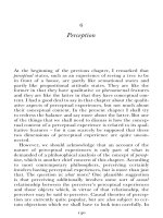
Each portfolio has an initial value and a final value or . Let us denote thepayoff
initial value of the two portfolios by and and the final values by ii i
EEßX
Fß!
,0
and . The values of Portfolio are shown in Figure 1. A similar figurei

FßX
E
holds for Portfolio .F
Introduction 7
time 0 time T
V
A,0
Possible
Values o
f
V
A,T
V
A,T
(
ω
1
)
V
A,T
(ω
2
)
V
A,T
(ω
n
)
Figure 1: The values of Portfolio E
As can be seen in the figure, Portfolio has a initial value . On theE known i

E,0
other hand, the final value of Portfolio is unknown at time . In fact, weE>œ!
assume that this value depends on the state of the economy at time , which canX
take one of possible values . Thus, the final value is actually a8ßáß== i
"8
EßX
function of these states. Similarly, we assume that the initial value of Portfolio F
is known and that the final value is a function of the possible states of the
economy.
Now, consider what happens if Portfolios and have exactly the sameEF
payoffs that is, ifregardless of the state of the economy;
i= i=
EßX
3FßX3
ÐÑœ ÐÑ
for all . The no-arbitrage pricing principle then implies that the3œ"ßáß8
initial values must be equal, that is
ii
Eß!
Fß!
œ
For suppose that . Then under the assumption of a perfect market, anii
Eß!
Fß!

investor can purchase the cheaper Portfolio and sell the more expensiveF
Portfolio , pocketing the positive difference . At time , EXii
Eß!
Fß!
no matter

what state the economy is in, the investor receives the common final value of the
portfolios and must pay out the same amount. Thus, he loses nothing at the end
and can keep the initial profit. This is arbitrage in the strongest sense, namely, a
guaranteed profit.
This approach can be used to determine an initial value of an asset, such as a
derivative, whose final payoff is known. To price the asset, all we need to do is
find a portfolio that has the same final payoff function as the asset we wish to
price, but has a known initial value. This is called a . Itreplicating portfolio
follows that the initial value of the asset in question must be equal to the initial
value of the replicating portfolio.
The no-arbitrage pricing principle can be used in other ways to determine prices.
For example, if the initial values of two portfolios are equal, then it cannot be
8 Introduction to the Mathematics of Finance
that one portfolio yields a higher payoff than the other, regardless of thealways
state of the economy.
We will see many examples of the use of the no-arbitrage pricing principle
throughout the book.
Miscellaneous Mathematical Facts
The Fundamental Counting Principle
Let be a sequence of tasks with the property that the number ofXßXßáßX
"# 5
ways to perform any task in the sequence does not depend on how the previous
tasks in the sequence were performed. Then, if there are ways to perform the8
3
3 X 3 œ "ß #ß á ß5th task , for all the number of ways to perform the entire
3
sequence of tasks is the product . For instance, if you are considering88â8
"# 5
buying one of five different stocks and one of six different bonds, then there are
&†'œ$! ways to buy one stock and one bond.

Permutations
Let be a set of size . An ordered arrangement of the elements of is called aW8 W
permutation of . The of each permutation is also . For example, thereW8size
are permutations of the set :'WœÖ+ß,ß-×
+,-ß+-,ß,+-ß,-+ß-+,ß-,+
More generally, an ordered arrangement of size of elements of is called5Ÿ8 W
a of size taken from . For instance, if , thenpermutation 5 W W œ Ö+ß,ß-ß.×
+., +and
are permutations of size . The number of permutations of a set is easily$
determined using the fundamental counting principle.
Theorem 1
1 The number of permutations of size is) 8
8x œ 8Ð8  "Ñâ# † "
The number is called . For consistency, we set .8x 8 !x œ "factorial
2 More generally, the number of permutations of size , taken from a set of) 5
size is8
8Ð8"ÑâÐ85"Ñœ
8x
Ð8  5Ñx
Proof. Part 1) is a special case of part 2), since taking in part 2) gives .5œ8 8x
As to part 2), there are ways to choose the first object in the8œ8!
permutation. Then there are choices for the second object, choices8" 8#