A Brief Introduction to Neural Networks doc
Bạn đang xem bản rút gọn của tài liệu. Xem và tải ngay bản đầy đủ của tài liệu tại đây (6.06 MB, 244 trang )
ABriefIntroductionto
NeuralNetworks
DavidKriesel
dkriesel.com
Downloadlocation:
/>NEW–fortheprogrammers:
ScalableandefficientNNframework,writteninJAVA
/>
dkriesel.com
In remembrance of
Dr. Peter Kemp, Notary (ret.), Bonn, Germany.
D. Kriesel – A Brief Introduction to Neural Networks (ZETA2-EN) iii
A small preface
"Originally, this work has been prepared in the framework of a seminar of the
University of Bonn in Germany, but it has been and will be extended (after
being presented and published online under www.dkriesel.com on
5/27/2005). First and foremost, to provide a comprehensive overview of the
subject of neural networks and, second, just to acquire more and more
knowledge about L
A
T
E
X . And who knows – maybe one day this summary will
become a real preface!"
Abstract of this work, end of 2005
The above abstract has not yet become a
preface but at least a little preface, ever
since the extended text (then 40 pages
long) has turned out to be a download
hit.
Ambition and intention of this
manuscript
The entire text is written and laid out
more effectively and with more illustra-
tions than before. I did all the illustra-
tions myself, most of them directly in
L
A
T
E
X by using XYpic. They reflect what
I would have liked to see when becoming
acquainted with the subject: Text and il-
lustrations should be memorable and easy
to understand to offer as many people as
possible access to the field of neural net-
works.
Nevertheless, the mathematically and for-
mally skilled readers will be able to under-
stand the definitions without reading the
running text, while the opposite holds for
readers only interested in the subject mat-
ter; everything is explained in both collo-
quial and formal language. Please let me
know if you find out that I have violated
this principle.
The sections of this text are mostly
independent from each other
The document itself is divided into differ-
ent parts, which are again divided into
chapters. Although the chapters contain
cross-references, they are also individually
accessible to readers with little previous
knowledge. There are larger and smaller
chapters: While the larger chapters should
provide profound insight into a paradigm
of neural networks (e.g. the classic neural
network structure: the perceptron and its
learning procedures), the smaller chapters
give a short overview – but this is also ex-
v
dkriesel.com
plained in the introduction of each chapter.
In addition to all the definitions and expla-
nations I have included some excursuses
to provide interesting information not di-
rectly related to the subject.
Unfortunately, I was not able to find free
German sources that are multi-faceted
in respect of content (concerning the
paradigms of neural networks) and, nev-
ertheless, written in coherent style. The
aim of this work is (even if it could not
be fulfilled at first go) to close this gap bit
by bit and to provide easy access to the
subject.
Want to learn not only by
reading, but also by coding?
Use SNIPE!
SNIPE
1
is a well-documented JAVA li-
brary that implements a framework for
neural networks in a speedy, feature-rich
and usable way. It is available at no
cost for non-commercial purposes. It was
originally designed for high performance
simulations with lots and lots of neural
networks (even large ones) being trained
simultaneously. Recently, I decided to
give it away as a professional reference im-
plementation that covers network aspects
handled within this work, while at the
same time being faster and more efficient
than lots of other implementations due to
1 Scalable and Generalized Neural Information Pro-
cessing Engine, downloadable at http://www.
dkriesel.com/tech/snipe, online JavaDoc at
the original high-performance simulation
design goal. Those of you who are up for
learning by doing and/or have to use a
fast and stable neural networks implemen-
tation for some reasons, should definetely
have a look at Snipe.
However, the aspects covered by Snipe are
not entirely congruent with those covered
by this manuscript. Some of the kinds
of neural networks are not supported by
Snipe, while when it comes to other kinds
of neural networks, Snipe may have lots
and lots more capabilities than may ever
be covered in the manuscript in the form
of practical hints. Anyway, in my experi-
ence almost all of the implementation re-
quirements of my readers are covered well.
On the Snipe download page, look for the
section "Getting started with Snipe" – you
will find an easy step-by-step guide con-
cerning Snipe and its documentation, as
well as some examples.
SNIPE: This manuscript frequently incor-
porates Snipe. Shaded Snipe-paragraphs
like this one are scattered among large
parts of the manuscript, providing infor-
mation on how to implement their con-
text in Snipe. This also implies that
those who do not want to use Snipe,
just have to skip the shaded Snipe-
paragraphs! The Snipe-paragraphs as-
sume the reader has had a close look at
the "Getting started with Snipe" section.
Often, class names are used. As Snipe con-
sists of only a few different packages, I omit-
ted the package names within the qualified
class names for the sake of readability.
vi D. Kriesel – A Brief Introduction to Neural Networks (ZETA2-EN)
dkriesel.com
It’s easy to print this
manuscript
This text is completely illustrated in
color, but it can also be printed as is in
monochrome: The colors of figures, tables
and text are well-chosen so that in addi-
tion to an appealing design the colors are
still easy to distinguish when printed in
monochrome.
There are many tools directly
integrated into the text
Different aids are directly integrated in the
document to make reading more flexible:
However, anyone (like me) who prefers
reading words on paper rather than on
screen can also enjoy some features.
In the table of contents, different
types of chapters are marked
Different types of chapters are directly
marked within the table of contents. Chap-
ters, that are marked as "fundamental"
are definitely ones to read because almost
all subsequent chapters heavily depend on
them. Other chapters additionally depend
on information given in other (preceding)
chapters, which then is marked in the ta-
ble of contents, too.
Speaking headlines throughout the
text, short ones in the table of
contents
The whole manuscript is now pervaded by
such headlines. Speaking headlines are
not just title-like ("Reinforcement Learn-
ing"), but centralize the information given
in the associated section to a single sen-
tence. In the named instance, an appro-
priate headline would be "Reinforcement
learning methods provide feedback to the
network, whether it behaves good or bad".
However, such long headlines would bloat
the table of contents in an unacceptable
way. So I used short titles like the first one
in the table of contents, and speaking ones,
like the latter, throughout the text.
Marginal notes are a navigational
aid
The entire document contains marginal
notes in colloquial language (see the exam-
Hypertext
on paper
:-)
ple in the margin), allowing you to "scan"
the document quickly to find a certain pas-
sage in the text (including the titles).
New mathematical symbols are marked by
specific marginal notes for easy finding
x
(see the example for x in the margin).
There are several kinds of indexing
This document contains different types of
indexing: If you have found a word in
the index and opened the corresponding
page, you can easily find it by searching
D. Kriesel – A Brief Introduction to Neural Networks (ZETA2-EN) vii
dkriesel.com
for highlighted text – all indexed words
are highlighted like this.
Mathematical symbols appearing in sev-
eral chapters of this document (e.g. Ω for
an output neuron; I tried to maintain a
consistent nomenclature for regularly re-
curring elements) are separately indexed
under "Mathematical Symbols", so they
can easily be assigned to the correspond-
ing term.
Names of persons written in small caps
are indexed in the category "Persons" and
ordered by the last names.
Terms of use and license
Beginning with the epsilon edition, the
text is licensed under the Creative Com-
mons Attribution-No Derivative Works
3.0 Unported License
2
, except for some
little portions of the work licensed under
more liberal licenses as mentioned (mainly
some figures from Wikimedia Commons).
A quick license summary:
1. You are free to redistribute this docu-
ment (even though it is a much better
idea to just distribute the URL of my
homepage, for it always contains the
most recent version of the text).
2. You may not modify, transform, or
build upon the document except for
personal use.
2 />by-nd/3.0/
3. You must maintain the author’s attri-
bution of the document at all times.
4. You may not use the attribution to
imply that the author endorses you
or your document use.
For I’m no lawyer, the above bullet-point
summary is just informational: if there is
any conflict in interpretation between the
summary and the actual license, the actual
license always takes precedence. Note that
this license does not extend to the source
files used to produce the document. Those
are still mine.
How to cite this manuscript
There’s no official publisher, so you need
to be careful with your citation. Please
find more information in English and
German language on my homepage, re-
spectively the subpage concerning the
manuscript
3
.
Acknowledgement
Now I would like to express my grati-
tude to all the people who contributed, in
whatever manner, to the success of this
work, since a work like this needs many
helpers. First of all, I want to thank
the proofreaders of this text, who helped
me and my readers very much. In al-
phabetical order: Wolfgang Apolinarski,
Kathrin Gräve, Paul Imhoff, Thomas
3 />neural_networks
viii D. Kriesel – A Brief Introduction to Neural Networks (ZETA2-EN)
dkriesel.com
Kühn, Christoph Kunze, Malte Lohmeyer,
Joachim Nock, Daniel Plohmann, Daniel
Rosenthal, Christian Schulz and Tobias
Wilken.
Additionally, I want to thank the readers
Dietmar Berger, Igor Buchmüller, Marie
Christ, Julia Damaschek, Jochen Döll,
Maximilian Ernestus, Hardy Falk, Anne
Feldmeier, Sascha Fink, Andreas Fried-
mann, Jan Gassen, Markus Gerhards, Se-
bastian Hirsch, Andreas Hochrath, Nico
Höft, Thomas Ihme, Boris Jentsch, Tim
Hussein, Thilo Keller, Mario Krenn, Mirko
Kunze, Maikel Linke, Adam Maciak,
Benjamin Meier, David Möller, Andreas
Müller, Rainer Penninger, Lena Reichel,
Alexander Schier, Matthias Siegmund,
Mathias Tirtasana, Oliver Tischler, Max-
imilian Voit, Igor Wall, Achim Weber,
Frank Weinreis, Gideon Maillette de Buij
Wenniger, Philipp Woock and many oth-
ers for their feedback, suggestions and re-
marks.
Additionally, I’d like to thank Sebastian
Merzbach, who examined this work in a
very conscientious way finding inconsisten-
cies and errors. In particular, he cleared
lots and lots of language clumsiness from
the English version.
Especially, I would like to thank Beate
Kuhl for translating the entire text from
German to English, and for her questions
which made me think of changing the
phrasing of some paragraphs.
I would particularly like to thank Prof.
Rolf Eckmiller and Dr. Nils Goerke as
well as the entire Division of Neuroinfor-
matics, Department of Computer Science
of the University of Bonn – they all made
sure that I always learned (and also had
to learn) something new about neural net-
works and related subjects. Especially Dr.
Goerke has always been willing to respond
to any questions I was not able to answer
myself during the writing process. Conver-
sations with Prof. Eckmiller made me step
back from the whiteboard to get a better
overall view on what I was doing and what
I should do next.
Globally, and not only in the context of
this work, I want to thank my parents who
never get tired to buy me specialized and
therefore expensive books and who have
always supported me in my studies.
For many "remarks" and the very special
and cordial atmosphere ;-) I want to thank
Andreas Huber and Tobias Treutler. Since
our first semester it has rarely been boring
with you!
Now I would like to think back to my
school days and cordially thank some
teachers who (in my opinion) had im-
parted some scientific knowledge to me –
although my class participation had not
always been wholehearted: Mr. Wilfried
Hartmann, Mr. Hubert Peters and Mr.
Frank Nökel.
Furthermore I would like to thank the
whole team at the notary’s office of Dr.
Kemp and Dr. Kolb in Bonn, where I have
always felt to be in good hands and who
have helped me to keep my printing costs
low - in particular Christiane Flamme and
Dr. Kemp!
D. Kriesel – A Brief Introduction to Neural Networks (ZETA2-EN) ix
dkriesel.com
Thanks go also to the Wikimedia Com-
mons, where I took some (few) images and
altered them to suit this text.
Last but not least I want to thank two
people who made outstanding contribu-
tions to this work who occupy, so to speak,
a place of honor: My girlfriend Verena
Thomas, who found many mathematical
and logical errors in my text and dis-
cussed them with me, although she has
lots of other things to do, and Chris-
tiane Schultze, who carefully reviewed the
text for spelling mistakes and inconsisten-
cies.
David Kriesel
x D. Kriesel – A Brief Introduction to Neural Networks (ZETA2-EN)
Contents
A small preface v
I From biology to formalization – motivation, philosophy, history and
realization of neural models 1
1 Introduction, motivation and history 3
1.1 Why neural networks? . . . . . . . . . . . . . . . . . . . . . . . . . . . . 3
1.1.1 The 100-step rule . . . . . . . . . . . . . . . . . . . . . . . . . . . 5
1.1.2 Simple application examples . . . . . . . . . . . . . . . . . . . . . 6
1.2 History of neural networks . . . . . . . . . . . . . . . . . . . . . . . . . . 8
1.2.1 The beginning . . . . . . . . . . . . . . . . . . . . . . . . . . . . 8
1.2.2 Golden age . . . . . . . . . . . . . . . . . . . . . . . . . . . . . . 9
1.2.3 Long silence and slow reconstruction . . . . . . . . . . . . . . . . 11
1.2.4 Renaissance . . . . . . . . . . . . . . . . . . . . . . . . . . . . . . 12
Exercises . . . . . . . . . . . . . . . . . . . . . . . . . . . . . . . . . . . . . . 12
2 Biological neural networks 13
2.1 The vertebrate nervous system . . . . . . . . . . . . . . . . . . . . . . . 13
2.1.1 Peripheral and central nervous system . . . . . . . . . . . . . . . 13
2.1.2 Cerebrum . . . . . . . . . . . . . . . . . . . . . . . . . . . . . . . 14
2.1.3 Cerebellum . . . . . . . . . . . . . . . . . . . . . . . . . . . . . . 15
2.1.4 Diencephalon . . . . . . . . . . . . . . . . . . . . . . . . . . . . . 15
2.1.5 Brainstem . . . . . . . . . . . . . . . . . . . . . . . . . . . . . . . 16
2.2 The neuron . . . . . . . . . . . . . . . . . . . . . . . . . . . . . . . . . . 16
2.2.1 Components . . . . . . . . . . . . . . . . . . . . . . . . . . . . . 16
2.2.2 Electrochemical processes in the neuron . . . . . . . . . . . . . . 19
2.3 Receptor cells . . . . . . . . . . . . . . . . . . . . . . . . . . . . . . . . . 24
2.3.1 Various types . . . . . . . . . . . . . . . . . . . . . . . . . . . . . 24
2.3.2 Information processing within the nervous system . . . . . . . . 25
2.3.3 Light sensing organs . . . . . . . . . . . . . . . . . . . . . . . . . 26
2.4 The amount of neurons in living organisms . . . . . . . . . . . . . . . . 28
xi
Contents dkriesel.com
2.5 Technical neurons as caricature of biology . . . . . . . . . . . . . . . . . 30
Exercises . . . . . . . . . . . . . . . . . . . . . . . . . . . . . . . . . . . . . . 31
3 Components of artificial neural networks (fundamental) 33
3.1 The concept of time in neural networks . . . . . . . . . . . . . . . . . . 33
3.2 Components of neural networks . . . . . . . . . . . . . . . . . . . . . . . 33
3.2.1 Connections . . . . . . . . . . . . . . . . . . . . . . . . . . . . . . 34
3.2.2 Propagation function and network input . . . . . . . . . . . . . . 34
3.2.3 Activation . . . . . . . . . . . . . . . . . . . . . . . . . . . . . . . 35
3.2.4 Threshold value . . . . . . . . . . . . . . . . . . . . . . . . . . . . 36
3.2.5 Activation function . . . . . . . . . . . . . . . . . . . . . . . . . . 36
3.2.6 Common activation functions . . . . . . . . . . . . . . . . . . . . 37
3.2.7 Output function . . . . . . . . . . . . . . . . . . . . . . . . . . . 38
3.2.8 Learning strategy . . . . . . . . . . . . . . . . . . . . . . . . . . . 38
3.3 Network topologies . . . . . . . . . . . . . . . . . . . . . . . . . . . . . . 39
3.3.1 Feedforward . . . . . . . . . . . . . . . . . . . . . . . . . . . . . . 39
3.3.2 Recurrent networks . . . . . . . . . . . . . . . . . . . . . . . . . . 40
3.3.3 Completely linked networks . . . . . . . . . . . . . . . . . . . . . 42
3.4 The bias neuron . . . . . . . . . . . . . . . . . . . . . . . . . . . . . . . 43
3.5 Representing neurons . . . . . . . . . . . . . . . . . . . . . . . . . . . . . 45
3.6 Orders of activation . . . . . . . . . . . . . . . . . . . . . . . . . . . . . 45
3.6.1 Synchronous activation . . . . . . . . . . . . . . . . . . . . . . . 45
3.6.2 Asynchronous activation . . . . . . . . . . . . . . . . . . . . . . . 46
3.7 Input and output of data . . . . . . . . . . . . . . . . . . . . . . . . . . 48
Exercises . . . . . . . . . . . . . . . . . . . . . . . . . . . . . . . . . . . . . . 48
4 Fundamentals on learning and training samples (fundamental) 51
4.1 Paradigms of learning . . . . . . . . . . . . . . . . . . . . . . . . . . . . 51
4.1.1 Unsupervised learning . . . . . . . . . . . . . . . . . . . . . . . . 52
4.1.2 Reinforcement learning . . . . . . . . . . . . . . . . . . . . . . . 53
4.1.3 Supervised learning . . . . . . . . . . . . . . . . . . . . . . . . . 53
4.1.4 Offline or online learning? . . . . . . . . . . . . . . . . . . . . . . 54
4.1.5 Questions in advance . . . . . . . . . . . . . . . . . . . . . . . . . 54
4.2 Training patterns and teaching input . . . . . . . . . . . . . . . . . . . . 54
4.3 Using training samples . . . . . . . . . . . . . . . . . . . . . . . . . . . . 56
4.3.1 Division of the training set . . . . . . . . . . . . . . . . . . . . . 57
4.3.2 Order of pattern representation . . . . . . . . . . . . . . . . . . . 57
4.4 Learning curve and error measurement . . . . . . . . . . . . . . . . . . . 58
4.4.1 When do we stop learning? . . . . . . . . . . . . . . . . . . . . . 59
xii D. Kriesel – A Brief Introduction to Neural Networks (ZETA2-EN)
dkriesel.com Contents
4.5 Gradient optimization procedures . . . . . . . . . . . . . . . . . . . . . . 61
4.5.1 Problems of gradient procedures . . . . . . . . . . . . . . . . . . 62
4.6 Exemplary problems . . . . . . . . . . . . . . . . . . . . . . . . . . . . . 64
4.6.1 Boolean functions . . . . . . . . . . . . . . . . . . . . . . . . . . 64
4.6.2 The parity function . . . . . . . . . . . . . . . . . . . . . . . . . 64
4.6.3 The 2-spiral problem . . . . . . . . . . . . . . . . . . . . . . . . . 64
4.6.4 The checkerboard problem . . . . . . . . . . . . . . . . . . . . . . 65
4.6.5 The identity function . . . . . . . . . . . . . . . . . . . . . . . . 65
4.6.6 Other exemplary problems . . . . . . . . . . . . . . . . . . . . . 66
4.7 Hebbian rule . . . . . . . . . . . . . . . . . . . . . . . . . . . . . . . . . 66
4.7.1 Original rule . . . . . . . . . . . . . . . . . . . . . . . . . . . . . 66
4.7.2 Generalized form . . . . . . . . . . . . . . . . . . . . . . . . . . . 67
Exercises . . . . . . . . . . . . . . . . . . . . . . . . . . . . . . . . . . . . . . 67
II Supervised learning network paradigms 69
5 The perceptron, backpropagation and its variants 71
5.1 The singlelayer perceptron . . . . . . . . . . . . . . . . . . . . . . . . . . 74
5.1.1 Perceptron learning algorithm and convergence theorem . . . . . 75
5.1.2 Delta rule . . . . . . . . . . . . . . . . . . . . . . . . . . . . . . . 75
5.2 Linear separability . . . . . . . . . . . . . . . . . . . . . . . . . . . . . . 81
5.3 The multilayer perceptron . . . . . . . . . . . . . . . . . . . . . . . . . . 84
5.4 Backpropagation of error . . . . . . . . . . . . . . . . . . . . . . . . . . . 86
5.4.1 Derivation . . . . . . . . . . . . . . . . . . . . . . . . . . . . . . . 87
5.4.2 Boiling backpropagation down to the delta rule . . . . . . . . . . 91
5.4.3 Selecting a learning rate . . . . . . . . . . . . . . . . . . . . . . . 92
5.5 Resilient backpropagation . . . . . . . . . . . . . . . . . . . . . . . . . . 93
5.5.1 Adaption of weights . . . . . . . . . . . . . . . . . . . . . . . . . 94
5.5.2 Dynamic learning rate adjustment . . . . . . . . . . . . . . . . . 94
5.5.3 Rprop in practice . . . . . . . . . . . . . . . . . . . . . . . . . . . 95
5.6 Further variations and extensions to backpropagation . . . . . . . . . . 96
5.6.1 Momentum term . . . . . . . . . . . . . . . . . . . . . . . . . . . 96
5.6.2 Flat spot elimination . . . . . . . . . . . . . . . . . . . . . . . . . 97
5.6.3 Second order backpropagation . . . . . . . . . . . . . . . . . . . 98
5.6.4 Weight decay . . . . . . . . . . . . . . . . . . . . . . . . . . . . . 98
5.6.5 Pruning and Optimal Brain Damage . . . . . . . . . . . . . . . . 98
5.7 Initial configuration of a multilayer perceptron . . . . . . . . . . . . . . 99
5.7.1 Number of layers . . . . . . . . . . . . . . . . . . . . . . . . . . . 99
5.7.2 The number of neurons . . . . . . . . . . . . . . . . . . . . . . . 100
D. Kriesel – A Brief Introduction to Neural Networks (ZETA2-EN) xiii
Contents dkriesel.com
5.7.3 Selecting an activation function . . . . . . . . . . . . . . . . . . . 100
5.7.4 Initializing weights . . . . . . . . . . . . . . . . . . . . . . . . . . 101
5.8 The 8-3-8 encoding problem and related problems . . . . . . . . . . . . 101
Exercises . . . . . . . . . . . . . . . . . . . . . . . . . . . . . . . . . . . . . . 102
6 Radial basis functions 105
6.1 Components and structure . . . . . . . . . . . . . . . . . . . . . . . . . . 105
6.2 Information processing of an RBF network . . . . . . . . . . . . . . . . 106
6.2.1 Information processing in RBF neurons . . . . . . . . . . . . . . 108
6.2.2 Analytical thoughts prior to the training . . . . . . . . . . . . . . 111
6.3 Training of RBF networks . . . . . . . . . . . . . . . . . . . . . . . . . . 114
6.3.1 Centers and widths of RBF neurons . . . . . . . . . . . . . . . . 115
6.4 Growing RBF networks . . . . . . . . . . . . . . . . . . . . . . . . . . . 118
6.4.1 Adding neurons . . . . . . . . . . . . . . . . . . . . . . . . . . . . 118
6.4.2 Limiting the number of neurons . . . . . . . . . . . . . . . . . . . 119
6.4.3 Deleting neurons . . . . . . . . . . . . . . . . . . . . . . . . . . . 119
6.5 Comparing RBF networks and multilayer perceptrons . . . . . . . . . . 119
Exercises . . . . . . . . . . . . . . . . . . . . . . . . . . . . . . . . . . . . . . 120
7 Recurrent perceptron-like networks (depends on chapter 5) 121
7.1 Jordan networks . . . . . . . . . . . . . . . . . . . . . . . . . . . . . . . 122
7.2 Elman networks . . . . . . . . . . . . . . . . . . . . . . . . . . . . . . . . 123
7.3 Training recurrent networks . . . . . . . . . . . . . . . . . . . . . . . . . 124
7.3.1 Unfolding in time . . . . . . . . . . . . . . . . . . . . . . . . . . . 125
7.3.2 Teacher forcing . . . . . . . . . . . . . . . . . . . . . . . . . . . . 127
7.3.3 Recurrent backpropagation . . . . . . . . . . . . . . . . . . . . . 127
7.3.4 Training with evolution . . . . . . . . . . . . . . . . . . . . . . . 127
8 Hopfield networks 129
8.1 Inspired by magnetism . . . . . . . . . . . . . . . . . . . . . . . . . . . . 129
8.2 Structure and functionality . . . . . . . . . . . . . . . . . . . . . . . . . 129
8.2.1 Input and output of a Hopfield network . . . . . . . . . . . . . . 130
8.2.2 Significance of weights . . . . . . . . . . . . . . . . . . . . . . . . 131
8.2.3 Change in the state of neurons . . . . . . . . . . . . . . . . . . . 131
8.3 Generating the weight matrix . . . . . . . . . . . . . . . . . . . . . . . . 132
8.4 Autoassociation and traditional application . . . . . . . . . . . . . . . . 133
8.5 Heteroassociation and analogies to neural data storage . . . . . . . . . . 134
8.5.1 Generating the heteroassociative matrix . . . . . . . . . . . . . . 135
8.5.2 Stabilizing the heteroassociations . . . . . . . . . . . . . . . . . . 135
8.5.3 Biological motivation of heterassociation . . . . . . . . . . . . . . 136
xiv D. Kriesel – A Brief Introduction to Neural Networks (ZETA2-EN)
dkriesel.com Contents
8.6 Continuous Hopfield networks . . . . . . . . . . . . . . . . . . . . . . . . 136
Exercises . . . . . . . . . . . . . . . . . . . . . . . . . . . . . . . . . . . . . . 137
9 Learning vector quantization 139
9.1 About quantization . . . . . . . . . . . . . . . . . . . . . . . . . . . . . . 139
9.2 Purpose of LVQ . . . . . . . . . . . . . . . . . . . . . . . . . . . . . . . . 140
9.3 Using codebook vectors . . . . . . . . . . . . . . . . . . . . . . . . . . . 140
9.4 Adjusting codebook vectors . . . . . . . . . . . . . . . . . . . . . . . . . 141
9.4.1 The procedure of learning . . . . . . . . . . . . . . . . . . . . . . 141
9.5 Connection to neural networks . . . . . . . . . . . . . . . . . . . . . . . 143
Exercises . . . . . . . . . . . . . . . . . . . . . . . . . . . . . . . . . . . . . . 143
III Unsupervised learning network paradigms 145
10 Self-organizing feature maps 147
10.1 Structure . . . . . . . . . . . . . . . . . . . . . . . . . . . . . . . . . . . 147
10.2 Functionality and output interpretation . . . . . . . . . . . . . . . . . . 149
10.3 Training . . . . . . . . . . . . . . . . . . . . . . . . . . . . . . . . . . . . 149
10.3.1 The topology function . . . . . . . . . . . . . . . . . . . . . . . . 150
10.3.2 Monotonically decreasing learning rate and neighborhood . . . . 152
10.4 Examples . . . . . . . . . . . . . . . . . . . . . . . . . . . . . . . . . . . 155
10.4.1 Topological defects . . . . . . . . . . . . . . . . . . . . . . . . . . 156
10.5 Adjustment of resolution and position-dependent learning rate . . . . . 156
10.6 Application . . . . . . . . . . . . . . . . . . . . . . . . . . . . . . . . . . 159
10.6.1 Interaction with RBF networks . . . . . . . . . . . . . . . . . . . 161
10.7 Variations . . . . . . . . . . . . . . . . . . . . . . . . . . . . . . . . . . . 161
10.7.1 Neural gas . . . . . . . . . . . . . . . . . . . . . . . . . . . . . . . 161
10.7.2 Multi-SOMs . . . . . . . . . . . . . . . . . . . . . . . . . . . . . . 163
10.7.3 Multi-neural gas . . . . . . . . . . . . . . . . . . . . . . . . . . . 163
10.7.4 Growing neural gas . . . . . . . . . . . . . . . . . . . . . . . . . . 164
Exercises . . . . . . . . . . . . . . . . . . . . . . . . . . . . . . . . . . . . . . 164
11 Adaptive resonance theory 165
11.1 Task and structure of an ART network . . . . . . . . . . . . . . . . . . . 165
11.1.1 Resonance . . . . . . . . . . . . . . . . . . . . . . . . . . . . . . . 166
11.2 Learning process . . . . . . . . . . . . . . . . . . . . . . . . . . . . . . . 167
11.2.1 Pattern input and top-down learning . . . . . . . . . . . . . . . . 167
11.2.2 Resonance and bottom-up learning . . . . . . . . . . . . . . . . . 167
11.2.3 Adding an output neuron . . . . . . . . . . . . . . . . . . . . . . 167
D. Kriesel – A Brief Introduction to Neural Networks (ZETA2-EN) xv
Contents dkriesel.com
11.3 Extensions . . . . . . . . . . . . . . . . . . . . . . . . . . . . . . . . . . . 167
IV Excursi, appendices and registers 169
A Excursus: Cluster analysis and regional and online learnable fields 171
A.1 k-means clustering . . . . . . . . . . . . . . . . . . . . . . . . . . . . . . 172
A.2 k-nearest neighboring . . . . . . . . . . . . . . . . . . . . . . . . . . . . 172
A.3 ε-nearest neighboring . . . . . . . . . . . . . . . . . . . . . . . . . . . . 173
A.4 The silhouette coefficient . . . . . . . . . . . . . . . . . . . . . . . . . . . 173
A.5 Regional and online learnable fields . . . . . . . . . . . . . . . . . . . . . 175
A.5.1 Structure of a ROLF . . . . . . . . . . . . . . . . . . . . . . . . . 176
A.5.2 Training a ROLF . . . . . . . . . . . . . . . . . . . . . . . . . . . 177
A.5.3 Evaluating a ROLF . . . . . . . . . . . . . . . . . . . . . . . . . 178
A.5.4 Comparison with popular clustering methods . . . . . . . . . . . 179
A.5.5 Initializing radii, learning rates and multiplier . . . . . . . . . . . 180
A.5.6 Application examples . . . . . . . . . . . . . . . . . . . . . . . . 180
Exercises . . . . . . . . . . . . . . . . . . . . . . . . . . . . . . . . . . . . . . 180
B Excursus: neural networks used for prediction 181
B.1 About time series . . . . . . . . . . . . . . . . . . . . . . . . . . . . . . . 181
B.2 One-step-ahead prediction . . . . . . . . . . . . . . . . . . . . . . . . . . 183
B.3 Two-step-ahead prediction . . . . . . . . . . . . . . . . . . . . . . . . . . 185
B.3.1 Recursive two-step-ahead prediction . . . . . . . . . . . . . . . . 185
B.3.2 Direct two-step-ahead prediction . . . . . . . . . . . . . . . . . . 185
B.4 Additional optimization approaches for prediction . . . . . . . . . . . . . 185
B.4.1 Changing temporal parameters . . . . . . . . . . . . . . . . . . . 185
B.4.2 Heterogeneous prediction . . . . . . . . . . . . . . . . . . . . . . 187
B.5 Remarks on the prediction of share prices . . . . . . . . . . . . . . . . . 187
C Excursus: reinforcement learning 191
C.1 System structure . . . . . . . . . . . . . . . . . . . . . . . . . . . . . . . 192
C.1.1 The gridworld . . . . . . . . . . . . . . . . . . . . . . . . . . . . . 192
C.1.2 Agent und environment . . . . . . . . . . . . . . . . . . . . . . . 193
C.1.3 States, situations and actions . . . . . . . . . . . . . . . . . . . . 194
C.1.4 Reward and return . . . . . . . . . . . . . . . . . . . . . . . . . . 195
C.1.5 The policy . . . . . . . . . . . . . . . . . . . . . . . . . . . . . . 196
C.2 Learning process . . . . . . . . . . . . . . . . . . . . . . . . . . . . . . . 198
C.2.1 Rewarding strategies . . . . . . . . . . . . . . . . . . . . . . . . . 198
C.2.2 The state-value function . . . . . . . . . . . . . . . . . . . . . . . 199
xvi D. Kriesel – A Brief Introduction to Neural Networks (ZETA2-EN)
dkriesel.com Contents
C.2.3 Monte Carlo method . . . . . . . . . . . . . . . . . . . . . . . . . 201
C.2.4 Temporal difference learning . . . . . . . . . . . . . . . . . . . . 202
C.2.5 The action-value function . . . . . . . . . . . . . . . . . . . . . . 203
C.2.6 Q learning . . . . . . . . . . . . . . . . . . . . . . . . . . . . . . . 204
C.3 Example applications . . . . . . . . . . . . . . . . . . . . . . . . . . . . . 205
C.3.1 TD gammon . . . . . . . . . . . . . . . . . . . . . . . . . . . . . 205
C.3.2 The car in the pit . . . . . . . . . . . . . . . . . . . . . . . . . . 205
C.3.3 The pole balancer . . . . . . . . . . . . . . . . . . . . . . . . . . 206
C.4 Reinforcement learning in connection with neural networks . . . . . . . 207
Exercises . . . . . . . . . . . . . . . . . . . . . . . . . . . . . . . . . . . . . . 207
Bibliography 209
List of Figures 215
Index 219
D. Kriesel – A Brief Introduction to Neural Networks (ZETA2-EN) xvii
Part I
From biology to formalization –
motivation, philosophy, history and
realization of neural models
1
Chapter 1
Introduction, motivation and history
How to teach a computer? You can either write a fixed program – or you can
enable the computer to learn on its own. Living beings do not have any
programmer writing a program for developing their skills, which then only has
to be executed. They learn by themselves – without the previous knowledge
from external impressions – and thus can solve problems better than any
computer today. What qualities are needed to achieve such a behavior for
devices like computers? Can such cognition be adapted from biology? History,
development, decline and resurgence of a wide approach to solve problems.
1.1 Why neural networks?
There are problem categories that cannot
be formulated as an algorithm. Problems
that depend on many subtle factors, for ex-
ample the purchase price of a real estate
which our brain can (approximately) cal-
culate. Without an algorithm a computer
cannot do the same. Therefore the ques-
tion to be asked is: How do we learn to
explore such problems?
Exactly – we learn; a capability comput-
ers obviously do not have. Humans have
Computers
cannot
learn
a brain that can learn. Computers have
some processing units and memory. They
allow the computer to perform the most
complex numerical calculations in a very
short time, but they are not adaptive.
If we compare computer and brain
1
, we
will note that, theoretically, the computer
should be more powerful than our brain:
It comprises 10
9
transistors with a switch-
ing time of 10
−9
seconds. The brain con-
tains 10
11
neurons, but these only have a
switching time of about 10
−3
seconds.
The largest part of the brain is work-
ing continuously, while the largest part of
the computer is only passive data storage.
Thus, the brain is parallel and therefore
parallelism
performing close to its theoretical maxi-
1 Of course, this comparison is - for obvious rea-
sons - controversially discussed by biologists and
computer scientists, since response time and quan-
tity do not tell anything about quality and perfor-
mance of the processing units as well as neurons
and transistors cannot be compared directly. Nev-
ertheless, the comparison serves its purpose and
indicates the advantage of parallelism by means
of processing time.
3
Chapter 1 Introduction, motivation and history dkriesel.com
Brain Computer
No. of processing units ≈ 10
11
≈ 10
9
Type of processing units Neurons Transistors
Type of calculation massively parallel usually serial
Data storage associative address-based
Switching time ≈ 10
−3
s ≈ 10
−9
s
Possible switching operations ≈ 10
13
1
s
≈ 10
18
1
s
Actual switching operations ≈ 10
12
1
s
≈ 10
10
1
s
Table 1.1: The (flawed) comparison between brain and computer at a glance. Inspired by: [Zel94]
mum, from which the computer is orders
of magnitude away (Table 1.1). Addition-
ally, a computer is static - the brain as
a biological neural network can reorganize
itself during its "lifespan" and therefore is
able to learn, to compensate errors and so
forth.
Within this text I want to outline how
we can use the said characteristics of our
brain for a computer system.
So the study of artificial neural networks
is motivated by their similarity to success-
fully working biological systems, which - in
comparison to the overall system - consist
of very simple but numerous nerve cells
simple
but many
processing
units
that work massively in parallel and (which
is probably one of the most significant
aspects) have the capability to learn.
There is no need to explicitly program a
neural network. For instance, it can learn
from training samples or by means of en-
n. network
capable
to learn
couragement - with a carrot and a stick,
so to speak (reinforcement learning).
One result from this learning procedure is
the capability of neural networks to gen-
eralize and associate data: After suc-
cessful training a neural network can find
reasonable solutions for similar problems
of the same class that were not explicitly
trained. This in turn results in a high de-
gree of fault tolerance against noisy in-
put data.
Fault tolerance is closely related to biolog-
ical neural networks, in which this charac-
teristic is very distinct: As previously men-
tioned, a human has about 10
11
neurons
that continuously reorganize themselves
or are reorganized by external influences
(about 10
5
neurons can be destroyed while
in a drunken stupor, some types of food
or environmental influences can also de-
stroy brain cells). Nevertheless, our cogni-
tive abilities are not significantly affected.
n. network
fault
tolerant
Thus, the brain is tolerant against internal
errors – and also against external errors,
for we can often read a really "dreadful
scrawl" although the individual letters are
nearly impossible to read.
Our modern technology, however, is not
automatically fault-tolerant. I have never
heard that someone forgot to install the
4 D. Kriesel – A Brief Introduction to Neural Networks (ZETA2-EN)
dkriesel.com 1.1 Why neural networks?
hard disk controller into a computer and
therefore the graphics card automatically
took over its tasks, i.e. removed con-
ductors and developed communication, so
that the system as a whole was affected
by the missing component, but not com-
pletely destroyed.
A disadvantage of this distributed fault-
tolerant storage is certainly the fact that
we cannot realize at first sight what a neu-
ral neutwork knows and performs or where
its faults lie. Usually, it is easier to per-
form such analyses for conventional algo-
rithms. Most often we can only trans-
fer knowledge into our neural network by
means of a learning procedure, which can
cause several errors and is not always easy
to manage.
Fault tolerance of data, on the other hand,
is already more sophisticated in state-of-
the-art technology: Let us compare a
record and a CD. If there is a scratch on a
record, the audio information on this spot
will be completely lost (you will hear a
pop) and then the music goes on. On a CD
the audio data are distributedly stored: A
scratch causes a blurry sound in its vicin-
ity, but the data stream remains largely
unaffected. The listener won’t notice any-
thing.
So let us summarize the main characteris-
tics we try to adapt from biology:
Self-organization and learning capa-
bility,
Generalization capability and
Fault tolerance.
What types of neural networks particu-
larly develop what kinds of abilities and
can be used for what problem classes will
be discussed in the course of this work.
In the introductory chapter I want to
clarify the following: "The neural net-
work" does not exist. There are differ-
Important!
ent paradigms for neural networks, how
they are trained and where they are used.
My goal is to introduce some of these
paradigms and supplement some remarks
for practical application.
We have already mentioned that our brain
works massively in parallel, in contrast to
the functioning of a computer, i.e. every
component is active at any time. If we
want to state an argument for massive par-
allel processing, then the 100-step rule
can be cited.
1.1.1 The 100-step rule
Experiments showed that a human can
recognize the picture of a familiar object
or person in ≈ 0.1 seconds, which cor-
responds to a neuron switching time of
≈ 10
−3
seconds in ≈ 100 discrete time
steps of parallel processing.
parallel
processing
A computer following the von Neumann
architecture, however, can do practically
nothing in 100 time steps of sequential pro-
cessing, which are 100 assembler steps or
cycle steps.
Now we want to look at a simple applica-
tion example for a neural network.
D. Kriesel – A Brief Introduction to Neural Networks (ZETA2-EN) 5
Chapter 1 Introduction, motivation and history dkriesel.com
Figure 1.1: A small robot with eight sensors
and two motors. The arrow indicates the driv-
ing direction.
1.1.2 Simple application examples
Let us assume that we have a small robot
as shown in fig. 1.1. This robot has eight
distance sensors from which it extracts in-
put data: Three sensors are placed on the
front right, three on the front left, and two
on the back. Each sensor provides a real
numeric value at any time, that means we
are always receiving an input I ∈ R
8
.
Despite its two motors (which will be
needed later) the robot in our simple ex-
ample is not capable to do much: It shall
only drive on but stop when it might col-
lide with an obstacle. Thus, our output
is binary: H = 0 for "Everything is okay,
drive on" and H = 1 for "Stop" (The out-
put is called H for "halt signal"). There-
fore we need a mapping
f : R
8
→ B
1
,
that applies the input signals to a robot
activity.
1.1.2.1 The classical way
There are two ways of realizing this map-
ping. On the one hand, there is the clas-
sical way: We sit down and think for a
while, and finally the result is a circuit or
a small computer program which realizes
the mapping (this is easily possible, since
the example is very simple). After that
we refer to the technical reference of the
sensors, study their characteristic curve in
order to learn the values for the different
obstacle distances, and embed these values
into the aforementioned set of rules. Such
procedures are applied in the classic artifi-
cial intelligence, and if you know the exact
rules of a mapping algorithm, you are al-
ways well advised to follow this scheme.
1.1.2.2 The way of learning
On the other hand, more interesting and
more successful for many mappings and
problems that are hard to comprehend
straightaway is the way of learning: We
show different possible situations to the
robot (fig. 1.2 on page 8), – and the robot
shall learn on its own what to do in the
course of its robot life.
In this example the robot shall simply
learn when to stop. We first treat the
6 D. Kriesel – A Brief Introduction to Neural Networks (ZETA2-EN)
dkriesel.com 1.1 Why neural networks?
Figure 1.3: Initially, we regard the robot control
as a black box whose inner life is unknown. The
black box receives eight real sensor values and
maps these values to a binary output value.
neural network as a kind of black box
(fig. 1.3). This means we do not know its
structure but just regard its behavior in
practice.
The situations in form of simply mea-
sured sensor values (e.g. placing the robot
in front of an obstacle, see illustration),
which we show to the robot and for which
we specify whether to drive on or to stop,
are called training samples. Thus, a train-
ing sample consists of an exemplary input
and a corresponding desired output. Now
the question is how to transfer this knowl-
edge, the information, into the neural net-
work.
The samples can be taught to a neural
network by using a simple learning pro-
cedure (a learning procedure is a simple
algorithm or a mathematical formula. If
we have done everything right and chosen
good samples, the neural network will gen-
eralize from these samples and find a uni-
versal rule when it has to stop.
Our example can be optionally expanded.
For the purpose of direction control it
would be possible to control the motors
of our robot separately
2
, with the sensor
layout being the same. In this case we are
looking for a mapping
f : R
8
→ R
2
,
which gradually controls the two motors
by means of the sensor inputs and thus
cannot only, for example, stop the robot
but also lets it avoid obstacles. Here it
is more difficult to analytically derive the
rules, and de facto a neural network would
be more appropriate.
Our goal is not to learn the samples by
heart, but to realize the principle behind
them: Ideally, the robot should apply the
neural network in any situation and be
able to avoid obstacles. In particular, the
robot should query the network continu-
ously and repeatedly while driving in order
to continously avoid obstacles. The result
is a constant cycle: The robot queries the
network. As a consequence, it will drive
in one direction, which changes the sen-
sors values. Again the robot queries the
network and changes its position, the sen-
sor values are changed once again, and so
on. It is obvious that this system can also
be adapted to dynamic, i.e changing, en-
vironments (e.g. the moving obstacles in
our example).
2 There is a robot called Khepera with more or less
similar characteristics. It is round-shaped, approx.
7 cm in diameter, has two motors with wheels
and various sensors. For more information I rec-
ommend to refer to the internet.
D. Kriesel – A Brief Introduction to Neural Networks (ZETA2-EN) 7