chemical equilibria and kinetics in soils
Bạn đang xem bản rút gọn của tài liệu. Xem và tải ngay bản đầy đủ của tài liệu tại đây (9.15 MB, 277 trang )
CHEMICAL
EQUILIBRIA
AND
KINETICS
IN
SOILS
CHEMICAL EQUILIBRIA
AND KINETICS IN
SOILS
Garrison Sposito
University
of
California
at Berkeley
New
York
Oxford
OXFORD
UNIVERSITY
PRESS
1994
Oxford University Press
Oxford New
York
Athens Auckland
Bangkok
Bombay
Calcutta Cape Town Dar es Salaam Delhi
Florence Hong Kong Istanbul Karachi
Kuala Lumpur Madras
Madrid
Melbourne
Mexico
City
Nairobi Paris Singapore
Taipei
Tokyo
Toronto
and
associated companies
in
Berlin Ibadan
Copyright © 1994 by
Oxford
University Press, Inc.
Published by Oxford University Press, Inc.,
200 Madison Avenue, New York. New
York
10016
Oxford is a registered trademark
of
Oxford University Press
All rights reserved. No part
of
this publication
may
be reproduced,
stored in a retrieval system, or transmitted, in any form or by any means,
electronic, mechanical, photocopying, recording,
or
otherwise,
without the prior permission
of
Oxford
University Press.
Library
of
Congress Cataloging-in-Publication
Data
Sposito, Garrison,
1939-
Chemical equilibria and kinetics in soils /
Garrison Sposito.
p. em. Rev. and
expanded
ed. of:
Thermodynamics
of
soil solutions. 1981.
Includes bibliographical references
and
index.
ISBN
0-19·507564-1
l.Soil
solutions. 2. Thermodynamics.
3. Chemical kinetics.
I.
Sposito, Garrison,
1939-
Thermodynamics
of
soil solutions.
II. Title
S592.5.S66 1994
63l.4'I-dc20
93-46714
'I X I h
~
.,
1'IIIIII'd
III
1111"
I
IlIIlt'l!
."Inll'
III
1\1111'111',1
1111
.II ,d 111'1'
Pill""
FOR
WERNER
STUMM
lux mentis lux orbis
PREFACE
Chemical thermodynamics is the theoretical structure on which the description
of
macroscopic assemblies
of
matter at equilibrium is based. This branch
of
physical chemistry was created 120 years ago by
Josiah
Willard Gibbs and
was perfected by the
1930's
through the work
of
G. N.
Lewis
and E.
A.
Ciuggenheim.
The
fundamental principles
of
the discipline thus have
long
heen established, and its scope as one
of
the five
great
subdivisions
of
physical science includes all the chemical
phenomena
that
material
systems
can exhibit in stable states.
It
is indeed powerful
enough
to provide unifying
principles for organizing and interpreting compositional
data
on natural
waters and soils. Although these data are known to
represent
only transitory
states
of
matter, characteristic
of
open systems in nature, they can be analyzed
III
a thermodynamic framework so long as the time scale
of
experimental
IIhservation
is
typically
incommensurable
with
the
time
scales
of
transformation among states
of
differing stability, a point stressed admirably
"lIlle 70 years ago by Gilbert Newton Lewis and
Merle
RandalJ.l
The
practitioners
of
chemical
thermodynamics
applied
to
soil
and
water
phenomena thereby have drawn success from an acute appreciation
of
the
lIatural time scales over which these
phenomena
take place and from a
pnceptive
intuition
of
how to make the "free-body cut": the
choice
of
a
dosed
model system whose behavior is to mimic an investigated open system
III
nature.
(i
i ven the firm status
of
chemical thermodynamics, its application to
dcserine chemical
phenomena
in soils would seem to be a straightforward
I'
\ncise,
hut experience has proven different. An obvious reason for the
dilliculties that have been encountered is the preponderant complexity
of
"lis. These multicomponent chemical systems comprise solid, liquid, and
)',I\COUS
phases that arc continually modified by the actions
of
biological,
itvdlldogical, and geological agents. In particular, the labile
aqueous
phase
III
~"il.
thc soil solution,
is
a dynamic, open, natural
water
system whose
'''I'IIl()sition
reflects
especially
the many
reactions
that
can
proceed
'''lIlIiltalll'ously hctwccn an aqucous solution and a lIIixturc
of
lIIincral and
vi
PREFACE
organic solids that
itself
varies both temporally and spatially.
The
net result
of
these reactions may be conceived as a dense web
of
chemical interrelations
mediated by variable fluxes
of
matter and energy from the atmosphere
and
biosphere.
It
is to this very complicated milieu that chemical thermodynamics
must
be applied.
An attempt to make this application prompted the appearance
of
The
Thermodynamics
of
Soil Solutions (Oxford University Press, 1981). Besides
its evident purpose, to demonstrate the use
of
chemical thermodynamics,
this
book
carried a leitmotif on the fundamental limitations
of
chemical
thermodynamics
for describing natural soils.
These
limitations
referred
especially to the influence
of
kinetics on stability, to the accuracy
of
thermodynamic
data,
and
to the
impossibility
of
deducing
molecular
mechanisms.
The
problem
of
mechanisms vis-a-vis thermodynamics
cannot
be expressed better than in the words
of
M.
L.
McGlashan:
2
"what
can we
learn from thermodynamic equations about the microscopic
or
molecular
explanation
of
macroscopic
changes?
Nothing
whatever.
What
is a
'thermodynamic
theory'?
(The phrase is used in the titles
of
many papers
published
in reputable chemical journals.) There is no such thing.
What
then is the use
of
thermodynamic equations to the chemist? THey are indeed
useful, but only by virtue
of
their use for the calculation
of
some desired
quantity which has not been measured,
or
which is difficult to measure,
from others which have been measured,
or
which are easier to measure."
This
point
cannot
be
stated often enough.
The
intervening years have brought the limitations as to kinetics and
mechanism into sharper focus, necessitating the present volume, which is a
revised and expanded textbook version
of
The Thermodynamics
of
Soil
Solutions. The need for revision was based especially on a growing awareness
that the quantitative description
of
soils in terms
of
the behavior
of
their
chemical
species
cannot
be
considered
complete
without
adequate
characterization
of
the rates
of
the chemical reactions they sustain. Full
recognition must be given and full account taken
of
the fact that few chemical
transformations
of
importance in natural soils go to completion exclusively
outside the time domain
of
their observation at laboratory or field scales. A
critical implication
of
this fact is that one
must
distinguish carefully between
thermodynamic
chemical
species,
sufficient
in
number
and
variety to
represent the stoichiometry
of
a chemical transformation between stable
states, and kinetic
chemical
species,
required
to
depict
completely
the
mechanisms
of
the transformation. The difficulty in bringing to fulfillment
the study
of
rate processes in natural systems derives from the fact that no
general laws
of
overall reaction kinetics exist in parallel with the general
laws
of
thermodynamics, and no necessary genetic relationship with which
to connect kinetic species to thermodynamic species
is
known. The resull
or
these conceptual lacunae
is
a largely empirical science
of
chcmical rate
processes,
at
timcs still rife with inadcquate theory and confusing data.
This
kxthook
i.~
intended primarily as a critical introduction to thl' use
of
chelllical thl'llllodynaillics and kinl'tlcs
101
(ksl'llhln~~
Il'al'llons
"'
thl'
PREFACE
vii
soil solution. Therefore no account is given
of
phenomena
in
the gaseous
and solid portions
of
soil unless they impinge directly on the properties
of
the aqueous phase, a restriction conducive to clarity in presentation and
relevance to the interests
of
most soil chemists. Although the discussion in
this
book
is self-contained,
it
does presume exposure to thermodynamics
and kinetics as taught in basic courses on physical chemistry. Since
most
of
the
examples
discussed
relate
to
soil
chemistry, a
background
in
that
discipline at the level
of
The Chemistry
of
Soils (Oxford University Press,
1989) will be
of
direct help in understanding the applications presented.
I should like to express my deep appreciation to William Casey, Wayne
Robarge, and Samuel Traina for their forthright, careful
review
of
the
manuscript for this book, and to Luc Derrendinger for his commentary on
Chapter 6.
Their
critical questions helped to exorcise numerous unclear
passages
and
errors in the text. Finally, I thank Mary Campbell-Sposito for
her assistance in preparing the index; Frank Murillo for his great skill in
drawing the figures; and Danny Heap, Joan
Van
Horn,
and
Terri
DeLuca
for
their patience in making a clear typescript from a great pile
of
handwritten
yellow sheets. None
of
these persons,
of
course, is responsible for errors
or
obscurities that may remain in this book. Each only deserves my gratitude
for keeping les sottises to a relative minimum.
NOTES
1.
G. N. Lewis and M. Randall, Thermodynamics
and
the Free Energy
of
Chemical Substances, McGraw-Hill, New York, 1923.
2.
M.
L.
McGlashan,
The
scope
of
chemical
thermodynamics,
Chemical
Thermodynamics, Spec. Periodical Rpt. 1: 1-30 (1973).
Ul'rkeley G. S.
January
1994
CONTENTS
1 Chemical Equilibrium
and
Kinetics 3
l.l
Chemical Reactions in Soil 3
1.2
The Equilibrium Constant 6
1.3
Reaction Rate Laws
12
1.4
Temperature Effects
16
1.5
Coupled Rate Laws
19
Special Topic
1:
Standard States
22
Notes
31
For
Further Reading
33
Problems
33
2 Chemical Speciation in Aqueous Solutions
37
2.1
Complexation Reactions 37
2.2 Oxidation-Reduction Reactions 49
2.3 Polymeric Species
60
.).4 Multispecies Equilibria 67
Special Topic
2:
Electrochemical Potentials 75
I. 1
1.2
I.
\
\-1
Notes 84
For
Further Reading 88
Problems 89
3
Mineral Solubility 93
Dissolution-Precipitation Reactions
93
Activity-Ratio and Predominance Diagrams
Mixed Solid Phases
113
Redllctivl' Dissolutioll Reactiolls 120
102
x CONTENTS
3.5 Dissolution Reaction Mechanisms 125
Notes
130
For
Further Reading 133
Problems 134
4
Surface
Reactions
138
4.1 Adsorption-Desorption Equilibria 138
4.2 Adsorption on Heterogeneous Surfaces 145
4.3 Adsorption Relaxation Kinetics 149
4.4 Surface Oxidation-Reduction Reactions 159
4.5 Transport-Controlled Adsorption Kinetics 166
Notes 171
For
Further Reading 175
Problems 176
5
Ion
Exchange
Reactions
181
5.1
Ion
Exchange as an Adsorption Reaction 181
5.2 Binary Ion Exchange Equilibria 187
5.3 Multicomponent Ion Exchange Equilibria 195
5.4
Ion
Exchange Kinetics 203
5.5 Heterogeneous Ion Exchange 208
Notes 214
For
Further Reading 216
Problems 217
6
Colloidal
Processes
222
6.1 Flocculation Pathways 222
6.2 The von Smoluchowski Rate Law
230
6.3 Scaling the von Smoluchowski Rate Law 238
6.4 Fuchsian Kinetics 243
6.5
The
Stability Ratio 249
Special Topic
3:
Cluster Fractals 253
Notes 257
For
Further Reading 261
Problems 261
Index 265
CHEMICAL
EQUILIBRIA
AND
KINETICS
IN
SOILS
d6d<;
dvro Kdtro ,.na
Kat
au't11
T.
S. Eliot
Burnt Norton
Je ne sais en
verite ce
qu'iljaut
Ie
plus admirer, de ['exces
de
bonte des hommes qui accueillent de si pauvres essais,
ou de mon incroyable assurance
a lancer
de
pareilles
sottices dans
Ie
monde.
Marcel Benabou
Pourquoi
je
n'
ai ecrit
aucun des mes livres
1
CHEMICAL
EQUILIBRIUM
AND
KINETICS
1.1 Chemical Reactions
in
Soils
Soils are multicomponent, multiphase, open systems that sustain a myriad
of
interconnected chemical reactions, including those involving the soil biota. The
multi phase nature
of
soil derives from its being a porous material whose void
spaces contain air and aqueous solution. The solid matrix (which itself
is
multiphase), soil air, and soil solution-each
is
a mixture
of
reactive chemical
compounds-hence the
multicomponent nature
of
soil. Transformations among
these compounds can be driven by flows
of
matter and energy to and from the
vicinal atmosphere, biosphere, and hydrosphere. These external flows,
as
well
as
the chemical composition
of
soil, vary in both space and time over a broad
range
of
scales.
The complexity
of
soil notwithstanding, the principal features
of
its chemical
behavior can
be
understood on the basis
of
well-established principles and
methods for the description
of
reactions in aqueous systems. Reactions that occur
exclusively in the gaseous phase or the solid matrix
of
soilless often control its
chemical behavior than reactions involving the aqueous phase. The basic
terminology associated with the latter chemical reactions will
be
reviewed in the
present chapter to provide an initial context for the discussion
of
equilibria and
kinetics to follow.
A chemical reaction
is
termed elementary
if
it occurs in a single step, with
no intermediate species appearing before the products
of
the reaction have
formed.
An
elementary reaction takes place on the molecular level exactly
as
written in terms
of
reactants and products. A reaction that
is
not elementary
is
composite or overall.!
An
example of an elementary reaction
is
the hydration
of
dissolved carbon dioxide in a soil solution to form the neutral species
H2CO~
("true carbonic acid"):
(1.1)
where aq refers
10
an
aqueous solulion phase and f
10
Ihe liquid phase.
In
this
4 CHEMICAL EQUILIDRIA AND KINETICS IN SOILS
elementary reaction, one
CO
2
molecule combines with one H
2
0 molecule
to
form directly one molecule
of
H
2
C0
3
.
The molecularity
of
this reaction is 2
(i.e., it is a bimolecular reaction), since that is the total number
of
reactant
species that come together
to
form the product. 1 This product, incidentally, is
to
be distinguished conceptually from "loosely solvated
COl>"
sometimes
denoted
as
a "species" by
CO
2
-H
2
0,
which,
at
equilibrium, makes up about
99.7%
of
the "nominal carbonic acid" (usually denoted H
2
CO;) in aqueous
solutions.
2
Another elementary reaction
of
molecularity 2 is the combination
of
true
carbonic acid with hydroxide ion
to
form bicarbonate ion and water:
(1.2)
Evidently, the overall reaction:
COiaq)
+ H
2
0(£)
W(aq) + HCO;-(aq) (1.3)
can be developed by adding the two elementary reactions in Eqs. 1.1 and 1.2 to
the elementary unimolecular reaction that describes the dissociation
of
the water
molecule:
(1.4)
The concept
of
molecularity thus is not applied to the reaction in Eq. 1.3, since
it does not display the actual molecular mechanism involving the intermediate
species,
H
2
COg,
OH-, and Hp. Therefore,
it
would be incorrect to interpret the
reaction in Eq. 1.3
as
the combination
of
one
CO
2
molecule with a water
molecule
to
form
H'
and
HCO;-
ions.
The error in this line
of
reasoning is
brought into sharper focus after noting that the elementary bimolecular reaction:
COiaq)
+ OW(aq)
HCO;-(aq) (1.5)
can be added
to
the elementary unimolecular reaction in Eq. 1.4 to produce
again the composite reaction in Eq. 1.3
by
a completely different pathway from
that obtained by the synthesis
of
Eqs. 1.1, 1.2, and 1.4. Experiment shows that
both pathways are operable in the pH range
8-10.
2
This example illustrates how
Eq. 1.3, like all other overall reactions, cannot be interpreted
prima facie in
molecular mechanistic terms. All that can be said is that 1 mol
CO
2
when
reacted with 1 mol
H
2
0 yields a mole each
of
protons and bicarbonate ions in
solution.
The development
of
chemical reactions
to
describe the transformations
of
material substances
and
the
determination
of
which chemical reactions are
elementary (i.e.,
the
determination
of
reaction mechanisms) arc principal
research
ohjectives
in
chemical science
and
in
soil
chemistry. Elementary
reactions arc always interpreted
at
the
lI10leclilar
level; therefore, experimental
CHEMICAL EQUILffiRIUM AND KINETICS
5
methods that probe at molecular space and time scales, notably spectroscopy,
must be applied to characterize reaction mechanisms.
By
contrast, overall
reactions have no unique molecular interpretation
and
therefore can be
investigated with macroscopic methods that provide information only about
changes in chemical composition
as
influenced, for
eXaIllple,
by temperature,
pressure,
or
time. The great complexity
of
soil chemical behavior has perforce
dictated that
most transformations
of
soil constituents be described by overall
reactions.
The rapid improvement in noninvasive spectroscopic techniques
during the past decades suggests, however, that ultirnatelyth
e
description
of
soil
chemistry in terms
of
elementary reactions
is
a realizable
goal.
This possibility
is
enhanced by the simplifying fact that all elementary reactions can be classified
as
acid-base (in the Lewis sense), oxidation-reduction,
or
free
radical reactions. 3
The reaction
of
dissolved CO
2
with hydroxide ions depicted in Eq. 1.4 takes
place entirely in the aqueous solution phase and
so
is
termed
homogeneous.
1
Another example
of
a homogeneous reaction
is
the formation
of
an outer-sphere
complex by
Mn
2
+ and CI- in a soil solution:
4
where
Mn
2
+(H
2
0)6 represents an octahedral solvation
complex
(inner-sphere) and
Mn2+(H20)6CI-
is an outer-sphere manganese-chloride
complex.
The weakly
associated chloride complex
is
proposed to transform to
an
inner-sphere chloride
complex by CI- exchange for a water molecule in the first solvation shell around
Mn
2
+:
5
This pair
of
homogeneous reactions can be added to derive
the
following overall
reaction:
(1.8)
ill which the water species are now suppressed to
emphasize
the overall nature
of
the complexation process depicted.
A reaction that involves chemical species in more
than
one
phase
is
termed
hl'ferogeneous.
1
An example
is
the composite reaction
describing
the reductive
dissolution
of
the common soil mineral hematite (a-FepJ) in the presence
of
visihle light by oxalic acid
(H
2
C
2
0
4
),
a ubiquitous
plant
litter degradation
product:
Fc
2
0J(s) I H
2
C
2
0laq)
I 4 H'(aq)
hv
-+
2 Fc
2
'(aq) I 2 COiaq)
13
H
2
0(1') (1.9)
whne
.\'
rcfer,~
to the solid phase
and
hv
denotes a
ljuantUlJlof
visihle I
iV-hI.
Tlw
6
CHEMICAL EQUILIDRIA AND KINETICS IN
SOILS
sequence
of
elementary reactions underlying this mineral dissolution process
is
a topic
of
current research. In one scenario
6
(Fig. 1.1), the oxalate anion forms
an inner-sphere complex with a Fe
3
+ cation exposed
at
the surface
of
the
mineral,
is
subsequently excited by a photon
of
visible light, transfers an
electron to the complexed Fe
3
+ ion
to
reduce it
to
Fe
2
+,
and finally decomposes
into
CO
2
species. The surface Fe
2
+ cation then detaches from the mineral
as
a
solvation complex and equilibrates with the aqueous solution phase
at
the
ambient pH value. This mechanistic sequence-which would be very different,
for example, in the absence of photons or in the presence of
oxygen-is
no
more
than implicit in Eq. 1.9. Without the underlying elementary reactions, Eq. 1.9
states simply that 1 mol hematite combined with 1 mol oxalic acid in the
presence
of
free protons can produce 2 mol Fe
2
+ and
CO
2
,
plus 3 mol water.
Macroscopic chemical techniques can
be
used
to
characterize overall
reactions like those in Eqs. 1.3, 1.8, and 1.9. Given the complexity
of
reaction
mechanisms, however, measurements
of
the composition
of
the aqueous system
in which an overall reaction occurs over the course
of
time may not always yield
data that conform
to
the expected stoichiometry. For example, if the reaction
of
carbon dioxide and water
to
produce protons and bicarbonate ions
is
initiated at
high pH (very low proton concentration), the disappearance
of
1 mol
CO
2
need
not be accompanied by the disappearance of 1 mol
H
2
0 (because
of
Eq. 1.5) or
by the appearance
of
1 mol
H+
(because
of
Eq.
1.1)Y
The unaccounted-for
presence
of
intermediate species (like
H2CO~
in Eq. 1.1) can lead typically to
a delay in the formation of one or more final product species relative
to
the
others, such that the expected stoichiometry in an overall reaction
is
violated
when the reaction progress
is
monitored. This transIent feature
of
mole balance
in overall reactions has important ramifications when the kinetics
of
soil
chemical processes are investigated (Section 1.3).
1.2 The Equilibrium Constant
If
the reactants and products in
Eq.
1.3
are
at
eqUilibrium, the reaction can be
expressed in the following equation:
COiaq)
+ H
2
0(£)
= W(aq) + HCO;(aq) (1.10)
where the equals sign signifies the equilibrium condition. A thermodynamic
equilibrium constant
can be defined for this reaction
at
a chosen temperature and
pressure, usually
25°C (298.15
K)
and 1 atm (101.325 kPa):
(1.11)
where boldface refers
to
the thermodynamic activity
of
the chemical species,
as
descrihed
in
Special Topic I
at
the end
of
this chapter. The parameter K
has
a
fixed value.
re~anl1ess
of
the colllPositioll
of
the soil solutioll.
To
make
this
CHEMICAL EQUILmRIUM AND KINETICS
7
hematite
oxalate
FIG.
1.1. A possible mechanism for the reductive dissolution
of
hematite by oxalic acid in the
presence
of
light (after Stumm et al."). See Section 3.4 for additional discussion
of
reductive
dissolution reactions.
assertion a reality, the activity
of
a species is related to its molality (moles
per
kilogram
of
water)
or
its concentration (in moles
per
cubic decimeter) through
all activity
('(}(~llicit'1lt:
8 CHEMICAL EQUILIDRIA AND KINETICS IN SOILS
(I) =
'Yi
[i]
(1.12)
where i is some chemical species, like
H+
or CO
2
,
of
concentration [z). The
activity coefficient
'Yi
has the units kg mol-
I
(or dm
3
mol-I), such that the activity
has
no units and the thermodynamic equilibrium constant is dimensionless (see
Special Topic 1).
Conventions and laboratory methods have been developed to measure
'Yi,
(i),
and K in aqueous solutions.
s
All species activity coefficients, for example, are
required to approach the value
1.0 (kg
mol-lor
dm
3
mol-I) when the species is
in its
Reference State. There are two principal definitions
of
the Reference State
for a solute in aqueous solution, like
H.,
HCO;,
and CO
2
in Eq. 1.10. One
is
the Infinite Dilution Reference State, wherein the activity coefficient
of
a solute
is defined to approach unit value
as
the concentration approaches zero for each
dissolved component
of
an aqueous solution at T = 298.15 K and P = 1 atm. The
other is the
Constant Ionic Medium Reference State, wherein the activity
coefficient
of
a solute approaches unit value
as
the concentration
of
only that
solute approaches zero, while the concentrations
of
all the other dissolved
components
of
the aqueous solution (the "background ionic medium") remain
fixed. Both definitions are valid thermodynamically, and each has advantages
and disadvantages. For example, in the case
of
the proton, the use
of
the
Constant Ionic Medium Reference State means that the activity coefficient
of
H +
in most soil solutions will very nearly have unit value and, therefore, that a
glass electrode will measure directly the proton
concentration in these solutions.
There is no need to calibrate the electrode against a set
of
standard buffer
solutions, since one may, in principle, simply make known additions
of
protons
to a reference solution and read the corresponding emf values
of
the electrode
in order to calibrate it.
On the other hand, this kind
of
calibration would have
to be done for every soil solution
of
interest instead
of
a single set
of
standard
buffer solutions (assuming that liquid junction potentials in the buffer solutions
are negligibly different from those in the soil solutions). The Infinite Dilution
Reference State usually
is
employed in this book. However, many published
thermodynamic properties
of
pure electrolyte solutions are based on the Constant
Ionic Medium Reference State (usually with
NaCI0
4
providing the background
ionic medium), and this choice
of
Reference State is popular among those who
study seawater and other saline natural waters whose composition does not vary
greatly.
Even with the definition
of
the Reference State, chemical thermodynamics
alone cannot provide a unique methodology for the measurement
of
single-ion
activity coefficients. An infinitude
of
possibilities exists, each
of
that calls upon
its own
extra thermodynamic set
of
conventions according to criteria
of
experimental convenience and intended application. However, chemical
thermodynamics does provide general constraints that limit any set
of
arbitrary
conventions defining single-ion activities.
'I
Consider
an
aq
lIeolis solut ion cont ai n i
n!!"
alllong ot
hers,
the
clect ro Iyte
M,,\.Io(aq),
where
M
rdt'rs
to a nwtal,
\.
rders
to a
ligand,
and
(/
and
I,
arc
CHEMICAL EQUILffiRIUM AND KINETICS
9
stoichiometric coefficients. The activity
of
the electrolyte
MaLt,
is
measurable by
well-established methods.
8,10
Experimental data pertaining to electrolyte activities
usually are catalogued in terms
of
the mean ionic activity coefficient 'Y
±:
10
(M
L)
=
",(a+b)m
a
m
b
ab
.±
TMTL
(1.13)
where m
TM
and m
TL
are total molalities
of
the metal and ligand, respectively,
If
only a single electrolyte were present in the aqueous solution to which 'Y ± refers,
then the product
of
molalities on the right side
of
Eq. 1.13 would reduce to a
power
of
the mean ionic molality;8
(1.14)
where m
T
is
the molality
of
the electrolyte, The molalities m
TM
,
m
TL
, and m
T
are
wholly macroscopic quantities that can be measured by standard spectroscopic,
complexometric, or gravimetric methods.
8
Thus
'Y ± can be calculated
unambiguously with Eq. 1.13 after the activity
of
the electrolyte
MaLt,(aq)
has
been determined.
It
is
evident that the mean ionic activity coefficient has a strict
chemical thermodynamic significance.
By
analogy with Eq. 1.13, one can define single-ion activity coefficients;9
(1.15)
where
'Y is a single-ion activity coefficient, m
M
is the molality
of
the species
Mm+(aq),
and m
L
is the molality
of
the species U-(aq).
For
'YM and 'YL to have
chemical significance, the species molalities, m
M
and m
L
,
must have a well-
defined operational meaning (see Section 2.4). Thus
the single-ion activity
coefficient has no meaning apart from the set
of
operational procedures used to
define ionic species
and
to determine their concentrations in an aqueous solution.
Although the left sides
of
Eqs. 1.13 and 1.15 always must be the same, it is not
possible in general to equate total molalities with species molalities, nor to
equate
'Y ± with hi'al'J
lI
(a+b),
The mean ionic and single-ion activity coefficients are conceptually different
parameters, but both must conform to the Debye-Hiickel infinite-dilution limit.
This theoretical constraint on activity coefficients takes on a particular
mathematical form, depending upon the way in which an electrolyte solution is
characterized. In a strictly thermodynamic picture
of
aqueous solutions, the
Debye-Hiickellimit can be expressed
as
follows;9
(1.16)
where
In
is
logarithm to the base e, p and q are the valences
of
M and L in Eq.
1.13,
All"
is
the Dehye-Hiickellimiting law parameter (AD" = 1.1762 kgl' mol-'h,
or
I ,1780
dm~12
mol
,/,
at
298
K).
The parameter
I.,
is
the stoichiometric ionic
.1'1
Tl'nxth;
10
CHEMICAL EQUlLmRIA AND KINETICS IN SOILS
(1.17)
where
Zi
is the valence
of
the metal
or
ligand whose total molality is m
Ti
and the
sum is over all metals (including hydrogen) and ligands (including hydroxide)
in solution. The Debye-Hiickellimit for the single-ion activity coefficients
of
an
electrolyte is similar to Eq.
1.16:
(1.18)
where
I.,f
is the effective ionic
strength:
(1.19)
In
Eq. 1.19, the sum is over all charged
species
in
the solution.
In
the limit
of
infinite dilution, soluble complexes should make a negligible contribution to
lef'
If
this is true, then Eqs. 1.16 and 1.18 can be combined into the following
single equation:
Lim
_1_
In[Y~Y~l
= Lim In Y ±
Ierl-0
a + b
I,~O
(1.20)
This equation represents a general theoretical constraint
on
single-ion activity
coefficients.
A general empirical constraint
on
single-ion activity coefficients also can be
imposed by means
of
Young's
rules.1O
For
dilute solutions,
Young's
rules are
equivalent to the statement that pairwise interactions between ions
of
opposite
charges make the dominant contribution to
'Y
±'
'YM'
and
'YL'
With respect to
'Y±,
this empirically based conclusion is often specialized to the Principle
of
Specific
Interaction.
10
Equations 1.16 and 1.18 are expressions
of
Young's
rules
in
the
Debye-Hiickellimit, in the sense that the ionic strength parameter accounts for
the effect
of
pairwise interactions between ions
of
opposite charge. At finite
ionic strength, Young's rules suggest that any mathematical expression for In
'Y
±
(or In
'YM
and In
'YL)
should include both linear and bilinear terms in the
molalities
of
all metals and ligands (or all charged species) in an aqueous
solution.
10
The Davies equation is a semiempirical expression for calculating single-ion
activity coefficients in soil solutions having effective ionic strengths up to about
0.5
mol kg-i. Other equations for
'YM
or
'YL
exist, but the Davies equation has the
distinct advantages
of
reliability in mixed electrolyte solutions and
of
exhibiting
only one adjustable parameter whose value is independent
of
the chemical nature
of
a charged species. The Davies equation for the activity coefficient
of
a
charged species J
is
expressed
as
follows:"
CHEMICAL
EQUILffiRIUM
AND
KINETICS
11
(1.21)
where
Zj
is the valence
of
species
1.
The adjustable parameter in the Davies
equation is the coefficient
of
lef'
which has the value
0.3A
DH
Zj.
For
uncharged monovalent metal-ligand complexes, proton-ligand com-
plexes (or dissolved gases), and bivalent metal-ligand complexes, some model
semiempirical equations for
"Yi
are the following:
11
-0.192I
ef
log Y
ML
= :: :-: , =:
0.0164 +
lef
(M = Na
+,
K"
etc.)
log
YHL
= O.lIef
(1.22)
(1.23)
(1.24)
for
lef
< 0.1 mol dm -
3
,
where log is logarithm to the base 10. These expressions
conform to a theoretical requirement for
neutral species, that log
"Y
become
proportional to
lef
in the infinite-dilution limit.
11
The expressions for single-species activity coefficients in Eqs.
1.21-1.24
suffice to calculate activities
of
dissolved solutes like
H+
or
CO
2
in Eq. 1.11.
For
the solvent, H
2
0,
it is still necessary to define a Reference State, which is that
of
the pure liquid at 298.15 K under 1 atm pressure.
12
The activity
of
the solvent
is
conventionally set equal to the product
of
a rational activity coefficient f and
the mole fraction
of
the solvent
X:
12
(1.25)
where x
H
0 is the ratio
of
the moles
of
water to the total moles
of
water and
solutes
iJ
an aqueous solution. For most soil solutions, x
H
0 z 1.0 and,
therefore, f
z 1.0, making
(H
2
0)
correspondingly close to
th€
value 1.0.
The combination
of
Eqs. 1.11 and 1.12 under the condition (H
2
0)
z 1
leads to the following expression:
K =
(II
+)(lICO~)/(COJ~O)
=
(II
+)(lICO~)/(COJ
=
yH[H
'le
YHea
[HCO;leIYco
[C0
2
l
e
J 2
==
(YHYHCO/Yco,)K
c
(1.26)
( 1 .27)
12 CHEMICAL EQUILffiRIA AND KINETICS
IN
SOILS
is
a conditional equilibrium constant for the reaction in Eq.
1.
10
and the
'Y
are
prescribed by Eqs.
1.21-1.24. The conditional equilibrium constant is defined
in terms
of
equilibrium species concentrations, [ 1
which makes it less abstract
than K in Eq.
1.
11, but also renders
it
composition dependent. Moreover,
Kc
has units (in this case, either molality or mol dm-
3
),
whereas K has no units.
The conceptual meaning
of
the activity
of
a chemical species stems from the
formal similarity between
K and
Kc.
The conditional equilibrium constant is a
more direct parameter with which to characterize equilibria, but it depends on
composition, in that it contains species concentrations only, and therefore it does
not correct for the interactions among species that occur
as
their concentrations
change. In the limit
of
infinite dilution, these interactions must die out, and the
extrapolated value
of
Kc
must represent chemical equilibrium in
an
ideal solution
wherein species interactions (other than those involved to form a complex like
HC0:J) are unimportant. The concentrations in
Kc
become equal numerically to
activities in the limit
of
either no interactions among species (Infinite Dilution
Reference State) or an invariant set
of
interactions among species (Constant
Ionic Medium Reference State). Thus the activity factors in K play the role
of
hypothetical concentrations
of
species
in
an ideal solution. But the real solution
is not ideal
as
species concentrations increase because the species are brought
closer together to interact more strongly. When this occurs,
Kc
must begin to
deviate from K. The activity coefficient
is
introduced to "correct" the
concentration factors in
Kc
for this nonideal species behavior and thereby restore
the value
of
K via Eq. 1.26. This correction is expected to be larger for charged
species than for neutral complexes (dipoles), and larger
as
the species valence
increases. These trends are reflected in the model expressions in Eqs.
1.21-1.24.
1.3 Reaction
Rate
Laws
For
the chemical reaction in Eq. 1.3, the extent
of
reaction
~
is defined by the
following differential expression:
1
(1.28)
where n is the number
of
moles
of
a substance and the assumption is made that
the reaction stoichiometry
is
known and
is
constant over the time period during
which the reaction is investigated. More generally,
if
A represents a reactant
with stoichiometric coefficient
-VA
and B represents a product with stoichiomet-
ric coefficient
VB'
then
( 1.29)
for any suhstances A and
B.
where
11"
</
()
and
li
ll
'
()
hy
II) PAC convellt
iOIl.
I
CHEMICAL EQUILIDRIUM AND KINETICS
13
In
Eq. 1.3,
UA
= -1 for any A and
UB
=
+1
for any
B.
Since Eq. 1.3 is an overall
reaction, the assumption
of
constant stoichiometry underlying the definition
of
~
is not trivial,
as
discussed in Section 1.1.
For
example, at high
pH,
Eq. 1.28
would not always be applicable because
of
the influence
of
the reactions in Eqs.
1.1 and 1.5. On the other hand, at equilibrium, when the hydration reaction is
described by Eq.
1.10, the application
of
Eq. 1.28 is possible. This fact serves
to emphasize the difference between
equilibrium chemical species that figure in
thermodynamic parameters (e.g., Eq. 1.11) and kinetic species that figure in the
mechanism
of
a reaction. The set
of
kinetic species is in general larger than the
set
of
equilibrium species for any overall chemical reaction.
The rate
of
conversion is the time derivative
of
the extent
of
reaction. I Thus
the rate is
d~
dt
-1 dnA
VA
dt
1
dn
B
VB
dt
(1.30)
for any substances A and B in a reaction.
If
the volume Y
of
the phase in which
a reaction occurs is constant, then I
yl
d~
= V 1
dC
A
dt dt
-1
dCB
VB
dt
(1.31)
is
the rate
of
reaction based on concentration, where c =
n/Y
is concentration. I
Sometimes the left side
of
Eq. 1.31 is also termed the rate
of
concentration
increase.
If
the volume Y is not constant
or
is not the volume
of
a particular
phase, the terms on the right side
of
Eq. 1.31 are expressed as
UAIy-1
dnAldt and
uBI
y-I
dnB/dt. This kind
of
generalization is needed for reactions occurring in
open systems
or
in multiphase systems (heterogeneous reactions). Note that the
rate
of
reaction has the same numerical value for all species involved,
as
long
as
Eq. 1.29 can be applied. Thus the rate
of
the reaction in Eq. 1.3 can be
measured by monitoring the moles
of
CO
2
,
water, protons,
or
bicarbonate over
time, as long as the stoichiometry
of
the reaction does not change.
The rate
of
a chemical reaction in aqueous solution typically is assumed to
depend in some way on the composition
of
the solution. As an example,
consider the following overall reaction to form a neutral sulfate complex with
a hivalent metal cation
as
the central group:
(1.32)
where the metal M can be Ca, Mg, Mn, Cu, etc. Detailed spectroscopic
Illvestigation shows that
MSO~(aq)
can be either an inner-
or
outer-sphere
(,()lI1plex.
with the latter species dominant. The rate
at
which
MSO~
forms
is
'1l1ile
high.
as
is
usual for metal ligand complexes.'
In
mathematical terms. this
laic
of
filflllation can
he
expressed
hy
the lime derivative
of
rMS()~/.
where. as
14
CHEMICAL EQUILffiRIA AND KINETICS
IN
SOILS
in Eq. 1.12, the square brackets represent a concentration in moles per liter
(moles per cubic decimeter). The rate
of
increase
of
soluble complex
concentration can be measured
by
a variety
of
spectroscopic and electrochemical
techniques.
5
,8
It
is common
to
assume that the observed rate can
be
represented
mathematically by the difference of two terms:
13
(1.33)
where R
f
and
Rb
each are functions of the composition
of
the solution in which
the reaction in Eq. 1.32 takes place,
as
well
as
of
the temperature and pressure.
Because the reaction in Eq. 1.32
is
not elementary, Eq. 1.33 need not have any
direct relationship
to
the molecular mechanism by which
MSO~
forms. For
example, there could be intermediate species that
do
not appear in the reaction
in Eq. 1.32 but that help to determine the observed rate and prevent it from
being a simple difference expression, Whenever Eq. 1.33
is
appropriate,
however, R
f
and
Rb
usually are interpreted
as
the respective rates
of
formation
("forward reaction") and dissociation ("backward reaction")
of
MSO~.
It
is
then
common
to
assume that R
f
depends on powers
of
the concentrations
of
the
reactants and that
Rb
depends on powers
of
the concentrations
of
the products:
13
(1.34)
where
kf'
kb'
a,
fl,
and 0
are
empirical parameters. The exponents
a,
fl,
and
a-which
need not
be
integers-are the partial orders
of
the reaction with
respect to the associated species [e.g.,
ath order with respect to M2+(aq)]. The
parameters k
f
and
kb
are the rate coefficients for the formation ("forward") and
dissociation
("backward") reactions, respectively. Each
of
the five parameters
in Eq. 1.34 may
be
functions
of
composition, temperature, and pressure.
1
Note
that the
SI
units
of
the rate coefficients will depend on the partial orders
of
the
reaction with respect
to
reactants or products and that there is no necessary
relationship between order and molecularity.
Equations 1.33 and 1.34 thus are
empirical models
of
the overall reaction rate whose relevance to molecular
mechanism must be demonstrated, not assumed. Any such model
of
an overall
reaction
is
required only to yield a positive rate when the direction
of
the
reaction
is
consistent with a decrease in Gibbs potential, and a zero rate when
chemical equilibrium
is
established.
13
Equation 1.34
is
an example
of
a reaction rate law. Its mathematical form
and five associated empirical parameters
are
objects for experimental study, To
facilitate this study.
Eg,
1.34
might
be
reformulated
as
the specific rate law:
CHEMICAL EQUILIDRIUM AND KINETICS
15
(1.35)
under the conditions that
(a)
the rate
of
dissociation
of
the complex is negligible;
(b) the reaction orders with respect to
M2+
and
SO~-
are the same
as
the
stoichiometric coefficients
of
these two species in Eq. 1.32; and (c)
[M2+]
=
[SO~T
The experimental value
of
k
f
now will have the units dm
3
mol-
1
S-l
and
the
overall order
of
the reaction
(==
ex
+
(3
in Eq.
1.
34) will be 2 [irrespective
of
assumption (c)]. Equation 1.35 can be simplified further and solved explicitly
for
[M2+]
as
a function
of
time
14
after rewriting the left side
as
-d[M2+]/dt (by
Eq. 1.32) and prescribing an initial condition on the concentration
of
M2+.
The
mathematical expression that results from solution then can be fitted to
experimental rate data in order to test Eq. 1.35 and determine the value
of
the
formation rate coefficient
k
f
•
Alternatively,
if
the reaction in Eq.
1.
32
is
at eqUilibrium, thereby
eliminating conditions (a) and (c), then the condition R
f
=
Rb
can be imposed
along with assumption
(b) (i.e.,
ex
=
(3
= 0 =
1)
and Eq. 1.34 leads to the
following expression:
(1.36)
as
applied to the reaction in Eq. 1.32, where [
]e
is
the concentration
of
a
species
at
equilibrium. The parameter
K,c
defined by the right side
of
Eq. 1.36
has
the units
of
inverse concentration and
is
the conditional stability constant for
Ihe
formation
of
the complex
MSO~.
It
is "conditional" because it is equal
numerically to
k/kb' a function
of
composition, temperature, and pressure.
Equation 1.36 shows that
K,c
can be calculated either with kinetics data (k
f
and
k
lo
) or with equilibrium data (the [ ]e). An alternative possibility is that one
of
Ihe
rate coefficients can be calculated by measuring the other rate coefficient
along with the equilibrium concentrations.
The facile line
of
reasoning that leads to Eqs. 1.33-1.36
is
so abundant in
Ihe
literature
of
soil chemical kinetics that the rather arbitrary nature
of
the
underlying assumptions often is
forgottenY For example, Eq. 1.36 is not a
unique consequence
of
Eq. 1.33.
If
the rate law
(1.37)
Wl're
10
replace Eq. 1.33, where p > 1 and gO
is
any positive-valued function
"I
species concentrations, then the direction
of
the arrow
in
Eq. 1.32 still would
11('
respecled and
Eq.
1.36 slill could
he
derived,
hUI
the rate
of
increase
of