reaction mechanisms of inorganic and organometallic systems (topics in inorganic chemistry)
Bạn đang xem bản rút gọn của tài liệu. Xem và tải ngay bản đầy đủ của tài liệu tại đây (27.43 MB, 532 trang )
Reaction Mechanisms
of
Inorganic
and
Organometallic
Systems
TOPICS
IN
INORGANIC CHEMISTRY
A
Series
of
Advanced
Textbooks
in
Inorganic Chemistry
Series
Editor
Peter
C.
Ford,
University
of
California, Santa Barbara
Chemical Bonding
in
Solids,
J.
Burdett
Reaction Mechanisms
of
Inorganic
and
Organometallic Systems,
3
rd
Edition,
R.
Jordan
Reaction Mechanisms
of
Inorganic
and
Organometallic
Systems
Third
Edition
Robert
B.
Jordan
OXFORD
UNIVERSITY
PRESS
2007
OXPORD
UNIVERSITY
PRESS
Oxford
University
Press,
Inc., publishes works that
further
Oxford
University's objective
of
excellence
in
research, scholarship,
and
education.
Oxford
New
York
Auckland
Cape Town
Dar es
Salaam Hong Kong Karachi
Kuala
Lumpur Madrid Melbourne Mexico City Nairobi
New
Delhi Shanghai Taipei Toronto
With
offices
in
Argentina
Austria Brazil Chile Czech Republic France Greece
Guatemala Hungary Italy Japan Poland Portugal Singapore
South Korea Switzerland Thailand Turkey Ukraine Vietnam
Copyright
©
2007
by
Oxford
University
Press, Inc.
Published
by
Oxford University Press, Inc.
198
Madison Avenue,
New
York,
New
York
10016
www.oup.com
Oxford
is a
registered trademark
of
Oxford University Press
All
rights reserved.
No
part
of
this publication
may be
reproduced,
stored
in a
retrieval system,
or
transmitted,
in any
form
or by any
means,
electronic, mechanical, photocopying, recording,
or
otherwise,
without
the
prior permission
of
Oxford University Press.
Library
of
Congress Cataloging-in-Publication Data
Jordan, Robert
B.
Reaction mechanisms
of
inorganic
and
organometallic systems
/
Robert
B.
Jordan.—3rd
ed
p.
cm.
Includes bibliographical references
and
index.
ISBN
978-0-19-530100-7
1.
Reaction mechanisms (Chemistry)
2.
Organometallic compounds.
3.
Inorganic
compounds.
I.
Title.
QD502J67
2006
41'.39—dc25
2006052498
987654321
Printed
in the
United States
of
America
on
acid-free paper
Preface
This book evolved
from
the
lecture notes
of the
author
for a
one-
semester
course given
to
senior undergraduates
and
graduate students
over
the
past
20
years. This third edition
presents
an
updating
of the
material
to
cover
the
literature through
to the end of
2005,
with
occasional excursions
to
early
2006.
As a
result,
the
total number
of
references
has
increased
from
about
660 in the
second edition
to
over
1570
in the
present one,
and 140
pages
of
text have been added; this
seems
to be a
clear testament
to the
vitality
of the
subject area.
A new
Chapter
9 on
kinetics
in
heterogeneous systems
has
been added. This
area
has
long been
the
domain
of
chemical engineers,
but it is of
increasing
relevance
to
inorganic kineticists
who are
studying catalytic
processes,
such
as
hydrogenation
and
carbonylation reactions, where
gas/liquid
mass transfer
is
involved. This chapter also covers
the
kinetic
aspects
of
adsorption
and
reaction
of
species
on
solids,
and the
question
of
whether
the
reaction
is
really homogeneous
or
heterogeneous.
The
overall organization
of the
first
edition
has
been retained.
The
first
two
chapters cover basic kinetic
and
mechanistic terminology
and
methodology. This material includes
new
sections
on the
analysis
of
data under second-order conditions, Curtin-Hammett conditions
and an
expanded discussion
of
pressure
effects.
New
material
has
been added
at
various
points throughout Chapters
3 and 4. The
coverage
of
organometallic
systems
in
Chapter
5 has
been increased substantially,
primarily
with
material
on
metal hydrides, catalytic hydrogenation
and
asymmetric
hydrogenation.
The
inverted region
and
activation
parameters
for
electron-transfer reactions predicted
by
Marcus theory
have been added
to
Chapter
6,
along with
an
expanded discussion
of
intervalence electron transfer.
The
recently revised assignment
of the
electronic spectra
of
metal carbonyls
has
resulted
in
substantial revisions
to
photochemical interpretations
in
Chapter
7. The
coverage
of
selected
bioinorganic systems
in
Chapter
8 has
been extended
to
include
methylcobalamin
as a
methyl transferase
and the
chemistry
of
nitric
oxide synthase. Chapter
10 on
experimental methods
and
their
applications
is
largely unchanged. Some
new
problems
for
each chapter
have been added.
There
is
more material than
can be
covered
in
depth
in one
semester,
but
the
organization allows
the
lecturer
to
omit
or
give less coverage
to
certain
areas
without jeopardizing
an
understanding
of
other areas.
It is
assumed that
the
students
are
familiar
with elementary crystal
field
v
vi Preface
theory
and its
applications
to
electronic spectroscopy
and
energetics,
and
concepts
of
organometallic chemistry, such
as the
18-electron rule,
71
bonding
and
coordinative unsaturation.
For the
material
in the
first
two
chapters, some background
from
a
physical chemistry course would
be
useful,
and
familiarity
with simple differential
and
integral calculus
is
assumed.
It is
expected
that students
will
consult
the
original literature
to
obtain
further
information
and to
gain
a
feeling
for the
excitement
in the
field.
This experience also should enhance their ability
to
critically evaluate
such work. Many
of the
problems
at the end of the
book
are
taken from
the
literature,
and
original references
are
given; outlines
of
answers
to
the
problems will
be
supplied
to
instructors
who
request them
from
the
author.
The
issue
of
units continues
to be a
vexing
one in
this area.
A
major
goal
of
this course
has
been
to
provide students with sufficient
background
so
that they
can
read
and
analyze current
research
papers.
To do
this
and be
able
to
compare results,
the
reader must
be
vigilant
about
the
units used
by
different authors. Energy units
are a
special
problem, since both joules
and
calories
are in
common usage. Both
units
have been retained
in the
text, with
the
choice made
on the
basis
of
the
units
in the
original work
as
much
as
possible. However, within
individual
sections
the
text uses
one
energy unit. Bond lengths
are
given
in
angstroms, which
are
still commonly quoted
for
crystal structures.
The
formulas
for
various calculations
are
given
in the
original
or
most
common format,
and
units
for the
various quantities
are
always
specified.
The
author
is
greatly indebted
to all of
those whose research efforts
have provided
the
core
of the
material
for
this book.
The
author
is
pleased
to
acknowledge those
who
have provided
the
inspiration
for
this
book: first,
my
parents,
who
contributed
the
early atmosphere
and
encouragement;
second,
Henry Taube, whose intellectual stimulation
and
experimental guidance ensured
my
continuing enthusiasm
for
mechanistic studies.
I am
only sorry that
I did not
finish
this edition
soon enough
for
Henry
to see
that
I did
make
the
changes
he
suggested.
Finally
and
foremost, Anna
has
been
a
vital force
in the
creation
of
this
book through
her
understanding
of the
time commitment,
her
comments, criticisms
and
invaluable editorial assistance
in
producing
the
camera-ready manuscript. However,
the
inevitable remaining
errors
and
oversights
are
entirely
the
responsibility
of the
author.
R.B.J.
Edmonton,
Alberta
June
2006
Contents
1
Tools
of the
Trade,
1
1.1
Basic Terminology,
1
1.2
Analysis
of
Rate Data,
3
1.3
Concentration Variables
and
Rate Constants,
12
1.4
Complex Rate Laws,
15
1.5
Complex Kinetic Systems,
15
1.6
Temperature Dependence
of
Rate Constants,
17
1.7
Pressure
Dependence
of
Rate Constants,
21
1.8
Ionic Strength Dependence
of
Rate Constants,
24
1.9
Diffusion-Controlled Rate Constants,
25
1.10 Molecular Modeling
and
Theory,
28
2
Rate
Law and
Mechanism,
31
2.1
Qualitative Guidelines,
31
2.2
Steady-State Approximation,
32
2.3
Rapid-Equilibrium Assumption,
34
2.4
Curtin-Hammett Conditions,
36
2.5
Rapid-Equilibrium
or
Steady-State?,
37
2.6
Numerical Integration Methods,
3 8
2.7
Principle
of
Detailed Balancing,
39
2.8
Principle
of
Microscopic Reversibility,
40
3
Ligand Substitution Reactions,
43
3.1
Operational Approach
to
Classification
of
Substitution Mechanisms,
43
3.2
Operational
Tests
for the
Stoichiometric Mechanism,
44
3.3
Examples
of
Tests
for a
Dissociative Mechanism,
49
3.4
Operational
Test
for an
Associative
Mechanism,
54
3.5
Operational
Tests
for the
Intimate Mechanism,
57
3.6
Some Special
Effects,
73
3.7
Variation
of
Substitution Rates
with
Metal Ion,
83
3.8
Ligand Substitution
on
Labile Transition-Metal Ions,
94
3.9
Kinetics
of
Chelate Formation,
100
4
Stereochemical Change,
114
4.1
Types
of
Ligand Rearrangements,
114
4.2
Geometrical
and
Optical Isomerism
in
Octahedral Systems,
119
4.3
Stereochemical Change
in
Five-Coordinate Systems,
128
4.4
Isomerism
in
Square-Planar Systems,
130
4.5
Fluxional Organometallic Compounds,
130
5
Reaction Mechanisms
of
Organometallic Systems,
150
5.1
Ligand Substitution Reactions,
150
5.2
Insertion Reactions,
168
5.3
Oxidative Addition Reactions,
177
vii
viii
Contents
5.4
Reductive Elimination Reactions,
188
5.5
Reactions
of
Alkenes,
188
5.6
Catalytic Hydrogenation
of
Alkenes,
195
5.7
Homogeneous Catalysis
by
Organometallic Compounds,
225
6
Oxidation-Reduction Reactions,
253
6.1
Classification
of
Reactions,
253
6.2
Outer-Sphere Electron-Transfer Theory,
256
6.3
Differentiation
of
Inner-Sphere
and
Outer-Sphere Mechanisms,
273
6.4
Bridging Ligand
Effects
in
Inner-Sphere Reactions,
274
6.5
Intervalence Electron Transfer,
281
6.6
Electron Transfer
in
Metalloproteins,
285
7
Inorganic Photochemistry,
292
7.1
Basic Terminology,
292
7.2
Kinetic Factors
Affecting
Quantum
Yields,
294
7.3
Photochemistry
of
Cobalt(III)
Complexes,
295
7.4
Photochemistry
of
Rhodium(III) Complexes,
301
7.5
Photochemistry
of
Chromium(III) Complexes,
304
7.6
Photochemistry
of
Ruthenium(II) Complexes,
310
7.7
Organometallic Photochemistry,
313
7.8
Photochemical Generation
of
Reaction Intermediates,
327
8
Bioinorganic Systems,
337
8.1. Basic Terminology,
337
8.2
Terms
and
Methods
of
Enzyme Kinetics,
338
8.3
Vitamin
B
12
,
341
8.4 A
Zinc(II) Enzyme: Carbonic Anhydrase,
356
8.5
Enzymic Reactions
of
Dioxygen,
361
8.6
Enzymic Reactions
of
Nitric Oxide,
373
9
Kinetics
in
Heterogeneous
Systems,
391
9.1
Gas/Liquid Heterogeneous Systems,
391
9.2
Gas/Liquid/Solid Heterogeneous Systems,
400
9.3
Where
is the
Catalyst?,
409
10
Experimental Methods,
422
10.1 Flow Methods,
423
10.2 Relaxation Methods,
428
10.3 Electrochemical Methods,
431
10.4 Nuclear Magnetic Resonance Methods,
435
10.5 Electron Paramagnetic Resonance Methods,
446
10.6 Pulse Radiolysis Methods,
448
10.7 Flash Photolysis Methods,
451
Problems,
457
Chemical Abbreviations,
488
Index,
491
Reaction Mechanisms
of
Inorganic
and
Organometallic
Systems
This page intentionally left blank
1
Tools
of the
Trade
This chapter covers
the
basic terminology
and
theory related
to the
types
of
studies that
are
commonly used
to
provide information about
a
reaction
mechanism.
The
emphasis
is on the
practicalities
of
determining rate
constants
and
rate laws. More background material
is
available
from
general physical chemistry texts
1,2
and
books devoted
to
kinetics.
3-5
The
reader
also
is
referred
to the
initial volumes
of the
series
edited
by
Bamford
and
Tipper.
6
Experimental techniques
that
are
commonly used
in
inorganic
kinetic
studies
are
discussed
in
Chapter
9.
1.1
BASIC TERMINOLOGY
As
with most fields,
the
study
of
reaction kinetics
has
some terminology
with
which
one
must
be
familiar
in
order
to
understand advanced books
and
research papers
in the
area.
The
following
is a
summary
of
some
of
these basic terms
and
definitions. Many
of
these
may be
known
from
previous studies
in
introductory
and
physical chemistry,
and
further
background
can be
obtained
from
textbooks devoted
to the
physical
chemistry
aspects
of
reaction kinetics.
Rate
For the
general reaction
the
reaction
rate
and the
rate
of
disappearance
of
reactants
and
rate
of
formation
of
products
are
related
by
In
practice,
it is not
uncommon
to
define
the
rate only
in
terms
of the
species
whose concentration
is
being monitored.
The
consequences that
can
result
from
different
definitions
of the
rate
in
relation
to the
stoichiometry
are
described below under
the
definition
of the
rate constant.
1
2
Reaction Mechanisms
of
Inorganic
and
Organometallic
Systems
Rate
Law
The
rate
law is the
experimentally determined dependence
of the
reaction
rate
on
reagent concentrations.
It has the
following
general form:
where
k is a
proportionality constant called
the
rate constant.
The
exponents
m and
n
are
determined experimentally
from
the
kinetic study
and
have
no
necessary relationship
to the
stoichiometric coefficients
in the
balanced chemical reaction.
The
rate
law may
contain
species
that
do not
appear
in the
balanced reaction
and may be the sum of
several terms
for
different
reaction pathways.
The
rate
law is an
essential piece
of
mechanistic information because
it
contains
the
concentrations
of
species necessary
to get
from
the
reactant
to
the
product
by the
lowest energy pathway.
A
fundamental
requirement
of
an
acceptable mechanism
is
that
it
must predict
a
rate
law
consistent
with
the
experimental rate law.
Order
of the
Rate
Law
The
order
of the
rate
law is the sum of the
exponents
in the
rate law.
For
example,
if m = 1 and n = -2 in Eq.
(1.3),
the
rate
law has an
overall order
of
-1.
However, except
in the
simplest
cases,
it is
best
to
describe
the
order
with
respect
to
individual reagents;
in
this example, first-order
in [A] and
inverse
second-order
in
[B].
Rate
Constant
The
rate constant,
k,
is the
proportionality constant that
relates
the
rate
to
the
reagent concentrations
(or
activities
or
pressures,
for
example),
as
shown
in Eq.
(1.3).
The
units
of k
depend
on the
rate
law and
must give
the
right-hand side
of Eq.
(1.3)
the
same units
as the
left-hand side.
A
simple example
of the
need
to
define
the
rate
in
order
to
give
the
meaning
of the
rate constant
is
shown
for the
reaction
If
the
experiment followed
the
rate
of
disappearance
of A,
then
the
experimental
rate
constant would
be 2k and it
must
be
divided
by 2 to get
the
numerical value
of k as
defined
by Eq.
(1.5).
However,
if the
formation
of B was
followed, then
k
would
be
determined directly from
the
experiment.
From
Eq.
(1.2),
and
assuming
the
rate
is
second-order
in
[A], then
Tools
of
the
Trade
3
Half-time
The
half-time, t
1/2
,
is the
time required
for a
reactant concentration
to
change
by
half
of its
total change. This term
is
used
to
convey
a
qualitative
idea
of the
time scale
for the
reaction
and has a
quantitative relationship
to
the
rate constant
in
simple cases.
In
complex systems,
the
half-time
may be
different
for
different
reagents
and one
should
specify
the
reagent
to
which
the
t
1/2
refers.
Lifetime
The
lifetime,
T, for a
particular species
is the
concentration
of
that species
divided
by its
rate
of
disappearance. This term
is
commonly used
in so-
called lifetime methods, such
as
NMR,
and in
relaxation methods, such
as
temperature jump.
1.2
ANALYSIS
OF
RATE
DATA
In
general,
a
kinetic study begins with
the
collection
of
data
of
concentration versus time
of a
reactant
or
product.
As
will
be
seen later,
this
can
also
be
accomplished
by
determining
the
time dependence
of
some
variable that
is
proportional
to
concentration, such
as
absorbance
or NMR
peak intensity.
The
next step
is to fit the
concentration-time
data
to
some
model that
will
allow
one to
determine
the
rate constant
if the
data
fits
the
model.
The
following section develops some integrated rate laws
for the
models
most commonly encountered
in
inorganic kinetics. This
is
essentially
a
mathematical problem; given
a
particular
rate
law as a
differential
equation,
the
equation must
be
reduced
to one
concentration variable
and
then
integrated.
The
integration
can be
done
by
standard methods
or by
reference
to
integration tables. Many more complex examples
are
given
in
advanced textbooks
on
kinetics.
1.2.1 Zero-Order Reaction
A
zero-order reaction
is
rare
for
inorganic reactions
in
solution
but is
included
for
completeness.
For the
general reaction
the
zero-order
rate
law is
given
by
and
integration
over
the
limits
[B] =
[B]
0
to [B] and t
=
0 to t
yields
4
Reaction Mechanisms
of
Inorganic
and
Organometallic
Systems
the
rate
of
disappearance
of A and
appearance
of B are
given
by
The
problem,
in
general,
is to
convert this
differential
equation
to a
form
with
only
one
concentration variable, either
[A] or
[B],
and
then
to
integrate
the
equation
to
obtain
the
integrated rate law.
The
choice
of the
variable
to
retain will depend
on
what
has
been measured experimentally.
One of the
concentrations
can be
eliminated
by
considering
the
reaction
stoichiometry
and the
initial conditions.
The
most general conditions
are
that
both
A and B are
present
initially
at
concentrations
[A]
0
and
[B]
0
,
respectively,
and
that
the
concentrations
at any
time
are
defined
as [A] and
[B].
For
this simple
case,
the
rate
law in
terms
of A can be
obtained
by
simple
rearrangement
to
give
This predicts that
a
plot
of [B] or [B] -
[B]
0
versus
t
should
be
linear with
a
slope
of k.
1.2.2
First-Order
Irreversible
System
Strictly
speaking, there
is no
such thing
as an
irreversible reaction.
It is
just
a
system
in
which
the
rate constant
in the
forward direction
is
much larger
than
that
in the
reverse direction.
The
kinetic analysis
of the
irreversible
system
is
just
a
special case
of the
reversible system that
is
described
in the
next
section.
For the
representative irreversible reaction
Then, integration over
the
limits
[A] =
[A]
0
to [A] and t = 0 to
/,
gives
and
predicts that
a
plot
of
In
[A]
versus
t
should
be
linear with
a
slope
of
-k\.
The
linearity
of
such plots
often
is
taken
as
evidence
of a
first-order
rate law. Since
the
assessment
of
linearity
is
somewhat subjective,
it is
better
to
show that
the
slope
of
such plots
is the
same
for
different
initial
concentrations
of A and
that
the
intercept corresponds
to the
expected
value
of
In
[A]
0
.
and it is now
common
to fit
data
to
this equation
by
nonlinear least squares
to
obtain
k\.
In
order
to
obtain
the
integrated
form
in
terms
of B, it is
necessary
to use
the
mass balance conditions.
For a 1:1
stoichiometry,
the
changes
in
concentration
are
related
by
Tools
of
the
Trade
5
The
equivalent exponential
form
of Eq.
(1.12)
is
At
the end of the
reaction,
[A] = 0 and [B] =
[B]^,
and
substitution
of
these
values into
Eq.
(1.14)
gives
After
rearrangement
of Eq.
(1.14)
and
substitution
from
Eq.
(1.15),
one
obtains
Then,
substitution
for [A]
from
Eq.
(1.16)
into
Eq.
(1.10)
gives
an
equation
that
can be
integrated over
the
limits
[B] =
[B]
0
to [B] and t - 0 to
t,
to
obtain
This
equation
also
can be
obtained
by
substitution
for
[A]
0
and [A]
from
Eq.
(1.15)
and
(1.16)
into
Eq.
(1.12)
and
predicts that
a
plot
of
In
([BL
-
[B])
versus
t
should
be
linear
with
a
slope
of
-k
v
The
half-time,
t
m
,
can be
obtained
from
Eq.
(1.12)
for the
condition
[A]
=
[A]</2,
or
from
Eq.
(1.17)
for [B] =
1/2([BL
-
[B]
0
)
+
[B]
0
.
In
either
case,
the
result
is
Therefore,
the
half-time
is
independent
of
the
initial concentrations.
An
important practical advantage
of the
first-order system
is
that
the
analysis
can be
done without
any
need
to
know
the
initial concentrations.
Therefore,
the
collection
of
concentration-time data
can be
started
at any
time arbitrarily defined
as t = 0.
This
is a
significant difference
from
the
second-order
case
that
is
described later
in
this chapter.
6
Reaction Mechanisms
of
Inorganic
and
Organometallic
Systems
1.2.3 First-Order Reversible System
For a
system coming
to
equilibrium, both
the
forward
and
reverse reactions
must
be
included
in the
kinetic analysis
and one
must take into account that
significant
concentrations
of
both reactants
and
products will
be
present
at
the end of the
reaction.
A
first-order system coming
to
equilibrium
may be
represented
by
The
rate
of
disappearance
of A
equals
the
rate
of
appearance
of B, and
these
are
given
by
Just
as
with
the
irreversible
system,
the
problem
is to
convert this
equation
to a
form
with only
one
concentration variable, either
[A] or
[B],
and
then integrate
the
equation
to
obtain
the
integrated rate law.
The
initial
concentrations
are
defined
as
[A]
0
and
[B]
0
,
those
at any
time
as [A] and
[B],
and the
final concentrations
at
equilibrium
as
[A]
e
and
[B]
e
.
Then,
mass balance gives
Note that
the
initial concentrations have been eliminated.
Since
Eq.
(1.24)
contains only
one
concentration variable, [B],
it can be
integrated directly. However,
it is
convenient
in the end to
eliminate
[A]
e
by
noting that,
at
equilibrium
the
rate
in the
forward direction must
be
equal
to the
rate
in the
reverse direction:
To
obtain
the
rate
law in
terms
of B, Eq.
(1.21)
can be
rearranged
to
obtain
the
following expressions
for [A] and
[A]
0
:
so
that
Substitution
for [A]
from
Eq.
(1.23) into
Eq.
(1.20)
gives
Tools
of
the
Trade
1
and
substitution
for
k,[A]
into
Eq.
(1.24)
gives
This equation
can be
rearranged
and
integrated over
the
limits
[B] =
[B]
0
to
[B]
and t = 0 to t to
obtain
Therefore,
a
plot
of
In
([B]
e
-
[B])
versus
t
should
be
linear
with
a
slope
of
-{fcj
+ fc_j).
Note that
the
kinetic study yields
the sum of the
forward
and
reverse rate constants.
If the
equilibrium constant,
K,
is
known, then
k
{
and
£_!
can be
calculated since
K =
kjk^.
Just
as in the
irreversible
first-order
system,
the
analysis
can be
done
without
any
need
to
know
the
initial
concentrations,
and the
collection
of
concentration-time data
can be
started
at any
time defined
as t - 0.
At
the
half-time,
t =
t
m
,
[B]
=
l/2([B]
e
-
[B]
0
)
+
[B]
0
,
and
substitution
intoEq.
(1.27)
gives
The
irreversible first-order system
is a
special
case
of the
reversible
system.
For the
irreversible system,
k
{
»
k_
{
so
that
(k
{
+
k_
l
)
=
k
l
.
1.2.4
Second-Order
Reversible
System
The
second-order
reversible system will
be
described
next
and the
simpler
irreversible system
will
be
developed later
as a
special
case
of the
reversible one. This reversible system
can be
described
by
where
b and c are
stoichiometric coefficients defined relative
to a
coefficient
of 1 for the
deficient reagent
A. The
rate
of
disappearance
of A
is
given
by
8
Reaction Mechanisms
of
Inorganic
and
Organometallic
Systems
It
will
be
assumed that there
is no C
present
initially
so
that mass balance
gives
the
concentrations
of B and C in
terms
of A as
Substitution
for [B] and [C]
from
Eq.
(1.31)
and for
k_
2
from
Eq.
(1.34)
into
Eq.
(1.30)
gives
the
following equation which
can be
integrated
because
[A] is the
only
concentration
variable:
and
at
equilibrium
It
is
convenient
to
eliminate
k_
2
before integrating
by
noting that
the
forward
and
reverse rates
are
equal
at
equilibrium:
which,
after rearrangement, gives
Integration over
the
limits
[A] =
[A]
0
to [A] and t - 0 to t
gives
the
following
solution:
A
plot
of the
first term
on the
left-hand
side
of Eq.
(1.36)
versus
t
should
be
linear with
a
slope related
to fc
2
, as
indicated
by the
right-hand side
of Eq.
(1.36).
It is
apparent that
one
must know
the
stoichiometry
coefficient,
b, in
addition
to the
initial concentrations,
[A]
0
and
[B]
0
,
and the
final
concentration,
[A]^
in
order
to do the
analysis
and to
determine
the
value
of
k
2
from
the
slope.
In
practice,
all of
these
requirements
can be
difficult
to
satisfy
so
that this
an
unpopular
and
uncommon situation
for
experimental
studies.
The
methods used
to
circumvent
these
requirements
are
described
in
Sections 1.2.6
and
1.2.8.
Tools of the Trade 9
1.2.5
Second-Order
Irreversible
System
This system
can be
obtained
as a
special case
of the
reversible system
by
simple consideration
of the
stoichiometry conditions.
If B is the
excess
reagent
and
reaction
(1.29)
goes essentially
to
completion, then
[A]
e
= 0,
and
substitution
of
this condition into
Eq.
(1.36) gives
In
this
case,
the
initial concentrations
of
both reactants
are
required
in
order
to
plot
the
first
term
on the
left
versus
t and to
determine
k
2
from
the
slope.
These
conditions
are not as
restrictive
as
those
for the
reversible second-
order
system,
but
they
are
still worse than those
for the
first-order system.
At
the
half-time
for
this second-order reaction,
[A]
=
[A]g/2,
and
substitution
into
Eq.
(1.37)
shows that
1.2.6
Pseudo-First-Order
Reaction
Conditions
The
pseudo-first-order reaction condition
is
very widely used,
but it is
seldom mentioned
in
textbooks. Although many reactions have second-
order
or
more
complex
rate
laws,
the
experimental kineticist wishes
to
optimize
experiments
by
taking advantage
of the
first-order rate
law
because
it
imposes
the
fewest restrictions
on the
conditions required
to
determine
a
reliable rate constant.
The
trick
is to use the
pseudo-first-order
condition.
The
pseudo-first-order condition requires that
the
concentration
of the
reactant whose concentration
is
monitored
is at
least
10
times smaller than
that
of all the
other reactants,
so
that
the
concentrations
of all the
latter
remain essentially constant during
the
reaction. Under this condition,
the
rate
law
usually simplifies
to a
first-order
form
and one
gains
the
advantage
of
not
needing
to
know
the
initial
concentration
of the
deficient reagent.
In the
preceding
irreversible
second-order example,
if it is
assumed that
the
conditions have been
set so
that
[B]
0
»[A]
0
,
then
[B]
0
»[C]
and
[C]
=
[A]
0
-
[A].
In
addition,
the
concentration
of B
will
remain constant
at
[B]
0
,
and the
final
concentration
of C is
[Ck
=
[A]
0
if the
reaction
is
irreversible
and has a
1:1
stoichiometry.
Substitution
of
these
conditions
intoEq.
(1.37)
gives
This equation predicts that
a
plot
of
In
([CL
-
[C])
versus
t
should
be
linear
10
Reaction
Mechanisms
of
Inorganic
and
Organometallic
Systems
with
a
slope
of
-fc
2
[B]
0
.
This
is
identical
in
form
to the
first-order
rate
law
except that
k\
is
replaced
by fc
2
[B]
0
- The
latter constant
is
often
called
the
observed,
£
obsd
,
or
experimental,
fc
exp
,
rate constant. Since
[B]
0
is
known,
it
is
possible
to
calculate
k
2
.
In
a
more general
case,
if the
rate
of
disappearance
of
reactant
A is a
function
of the
concentrations
of
other species
X, Y and Z,
then
the
rate
of
disappearance
of A may be
given
by
If
the
conditions
are
such that
[X]
0
,
[Y]
0
,
[Z]
0
»
[A],
so
that [X],
[Y] and
[Z]
remain essentially constant, then
and the
rate
law has the
first-order
form.
1.2.7 Comparison
of
First-Order
and
Second-Order Conditions
The
differences between second-order
and
first-order kinetic behavior,
and
the
transition
from
second-order
to
pseudo-first-order conditions
are
illustrated
by the
curves
in
Figure
1.1.
These
curves
are
based
on the
system
and
show
the
time dependence
of the
formation
of C. The
deficient reagent
is
A,
with
[A]
0
=
0.10
M,
different
initial
concentrations
of B of
0.50, 0.70,
0.85
and 1.0 M are
used,
and
k
2
=
3xlO"
3
M~
!
s
-1
.
The
lower curve, with
[B]
0
=
0.50
M,
represents
a
typical time dependence
for
second-order
conditions. Note that this time dependence
has a
more gradual approach
to
the
final
value than
the
others
in
Figure 1.1. Thus,
a
qualitative
examination
can
provide
an
indication
of the
second-order nature
of the
reaction.
The
fact
that
the
rate
is
slower under second-order conditions
can
be
used
to
advantage
if the
limits
of the
experimental method
are
being
strained.
As
[B]
0
is
increased,
C is
formed more rapidly
and the
curves approach
a
first-order shape. When
[B]
0
= 1.0 M,
[B]
0
>
10[A]
0
and the
pseudo-first-
order condition
has
been reached. Then,
the
curve calculated
from
Eq.
(1.37)
for
second-order conditions
is
almost indistinguishable
from
the
line
calculated
from
Eq.
(1.39)
for
pseudo-first-order conditions.
The
correspondence
of
these curves
is the
rationale
for the
general rule that
pseudo-first-order conditions require
at
least
a
10-fold
excess
of the
reagents
whose concentrations
are to
remain constant.
Tools
of
the
Trade
11
Figure 1.1.
The
time
dependence
for
formation
of
product
C
with
the
initial
deficient
reagent
[A]
0
=
0.10
M.
Results
are
calculated
for
pseudo-first-order
(—)
conditions
and
concentrations
(M) of the
excess reagent
B of
0.50 (•), 0.70
(n),
0.85 (•),
l.O(o).
1.2.8 Initial Rate Method
This
is a
method
for
determining
the
concentration dependence
of a
rate
law
that avoids
the
need
for an
integrated rate
law or
pseudo-first-order
conditions.
It is
based
on the
assumption that
the
reactant concentrations
are
essentially constant during
the
initial
-10%
of
reaction.
The use of
this
method requires that observation
can
begin very soon after mixing
the
reactants
and
that
the
detection method
is
sensitive enough
to
provide
precise data over
the
small extent
of
reaction.
The
latter condition usually
means that
the
reaction half-time
is
about
ten
seconds
or
longer,
so
that this
method
is
convenient
and
efficient
for
slow reactions. Observation over
a
short initial period
may
avoid,
but
also
may
hide, kinetic
and
chemical
complications that only
are
clearly apparent later
in the
reaction.
The
kinetic runs simulated
in
Figure
1.2 are for a
second-order
rate
law
with
varying initial concentrations
of the
reactants
A and B,
with
A as the
deficient
reagent.
The
absorbance,
7
A
,
which
is
proportional
to the
concentration
of A, has
been measured
at 2 s
intervals.
For
illustrative
purposes,
the
concentrations have been chosen
so
that
the
initial
rate,
£
2
[A]
0
[B]
0
,
is the
same
for all the
runs. More commonly,
the
reagent
concentrations
are
varied
one at a
time
in a
series
of
kinetic runs
in
order
to
determine
the
rate law.
12
Reaction
Mechanisms
of
Inorganic
and
Organometallic
Systems
Figure
1.2.
The
time dependence
of the
absorbance,
/
A
,
of
reactant
A
during
the
initial
stages
of its
reaction
with
B
with
a
rate
law
-d[A]/df
=
£
2
[A][B]
and
k
2
=
3.0xl(T
2
NT
1
s'
1
.
Initial
concentrations
(M)
are:
[A]
0
=
0.050,
[B]
0
=
0.400
(o);
[A]
0
=
0.033,
[B]
0
=
0.600 (o);
[A]
0
=
0.020,
[B]
0
= 1.0
(o).
The
simplest
way of
determining
the
initial rate
is to
take
the
slopes
of
the
lines through
the
initial points,
as
shown
in
Figure 1.2. Strictly
speaking,
the
slopes should
be
taken
for
lines which cover
the
same extent
of
reaction
but
this
is not
always obvious when
one
just observes
a
small
portion
of the
reaction.
In the
Figure,
the
more common practice
of
taking
the
slope over
a
fixed time
is
illustrated, even though
the
extent
of
reaction
is
greatest
for the
fastest (lower) data set.
As a
result,
the
slopes actually
range
from
0.103
to
0.112
s'
1
,
although they should
be
equal.
In
this
case,
the
error
probably
is not too
significant
for the
purpose
of
determining
the
rate law. This
difficulty
can be
minimized
by
fitting
the
data over
a
greater
extent
of the
reaction
to a
power series
in
t,
such
as
7,
=
/
0
+ at +
P*
2
,
in
which
case
a
will
be the
initial slope.
In
order
to
determine
the
actual rate
constant,
one
must know
the
relationship between
the
property being
observed
and the
concentration.
1.3
CONCENTRATION VARIABLES
AND
RATE CONSTANTS
The
rate laws have been developed
in
terms
of
concentrations,
but in
many
cases
it is not
practical
or
possible
to
determine actual molar concentrations
as a
function
of
time. However,
it is
easy
to
measure some property that
is
Tools
of
the
Trade
13
known
to be
directly proportional
to
molar concentration, such
as
absorbance
in the
electronic
or
infrared spectrum,
NMR
integrated peak
intensity,
conductance
or
refractive index.
The
following development shows
the
general relationship between
the
concentration
of the
limiting reagent
and the
property being measured
for
the
irreversible reaction
The
equation
is
balanced
so
that
A has a
coefficient
of 1 in
order
to
simplify
the
ratios
bla,
yla
and
z/a
which otherwise would appear
in the
equations.
The
property being
measured
is
designated
as / and its
proportionality constant
with
concentration
is e. At any
time,
the
value
of /
is
given
by
and
the
initial value
is
given
by
If
A is the
limiting reagent, then
the
final
value
of / is
given
by
The
following
stoichiometric
relationships
can be
used
to
express
the
concentrations
of B, Y and Z in
terms
of A:
Substitution
of
these values into
Eq
(1.44)
gives
Then,
taking
the
difference
/,
-
/„
and
solving
for
[A]
gives
Similarly,
7
0
-
/^
gives
[A]
0
as
14
Reaction Mechanisms
of
Inorganic
and
Organometallic Systems
Combination
of the
last
two
equations gives
Substitution
for [A]
into
the
integrated rate
law
gives equations
that
can be
used
to
determine
a k
from
measurements
of /.
1.3.1 First-Order Irreversible System
A
simple rearrangement
of the
previous solution
for
this system
(Eq.
(1.12))
and
substitution
for [A] and
[A]
0
from
Eq.
(1.49)
and
(1.50)
gives
This shows that
a
plot
of
In
(/,
-
/„)
versus
t
should
be
linear with
a
slope
of
-fc,.
It is not
necessary
to
know
the
concentration
of A or any
values
of e in
order
to
determine
the
rate constant,
but one
does need
/.„.
Sometimes,
it is
impossible
to
measure
/„,,
because
of
secondary reactions,
or it is
inconvenient
because
the
reaction
is
slow. Such systems
can be
analyzed
by
nonlinear least-squares fitting
of the
data over
as
much
of the
reaction
as
possible,
or in a
more classical
way by the
Guggenheim method,
described
in
more detail
by
Moore
and
Pearson
3
(p
71),
Mangelsdorf
7
and
Espenson
8
(p
25).
1.3.2 Second-Order Irreversible System
The
integrated rate
law for
this system
is
given
by Eq.
(1.37)
which
may be
rewritten
as
Then, substitution
for [A] from Eq.
(1.51)
gives
Therefore,
a
plot
of the
first
term
on the
left-hand
side versus
t
should
be
linear with
a
slope
of
([B]
0
-
fe[A]
0
)fc
2
.
Clearly
in
this
case,
it is
necessary
to
know
the
stoichiometry
coefficient,
b,
as
well
as the
initial concentrations,
[B]
0
and
[A]
0
,
in
order
to
determine
k
2
.
However, only
b and the
ratio
of
[B]
0
to
[A]
0
are
needed
in
order
to
make
the
plot.