modern control engineering, 4th edtion (2002)- ogata

Modern Contro
Engineering
a
Fourth Edition
Katsuhiko Ogata
University of Minnesota
Pearson Education International
-
Ogata. Kafsutuko
Modern
Control Engineering
I
Katsuiko 0gata
4
th
cd,
-
Ned
3
e75Cd
:
Tehran:
A'eizh
1381
=
2002.
964
P.:
iU
Catalogmg

based
on
CIP
information.
Reprint
of
4th
cd.,
UX12
Prentiffi Hall,
New
Jmey,
ISBN
0-13-043245-8.
1
.
A
3
to
ma+;
c
w
n
L
-
'3.
Wml
Enginaring
2
Control

?henry
L
TIUe.
Modem
Control
Engineering.
TJ
213
A7
M2
69818
2002
National
lib. of Iran
MS1-12481
Book
Name
:
Madern
Control
Enginring
by
:
Katsuhiko
Ogata
Publisher
:
Aeeizb
Lithopraphy
!

Norang
Printing
&
bookbinding
:
Pezhman
Srze
:
205.225
Time
&
date
of
1st
print
:
Fall,
1381
(2002)
Number
:
1500
Number
of Pages
:
976
DISTRIBUTORS
KETABlRAN
:
PHONE

NO
:
021- 6423416, 021
-
6926687
NOPARDAZAN
:
PHONE
NO
:
021
-
6411173,
021
-
6494409
This edition may be sold only in those countries
to which it
is
consigned by Pearson Education International.
It is not to be re-exported and it is not for sale
in the
U.S.A., Mexico, or Canada.
Vice President and Editorial Director, ECS:
Marcia
J;
Horton
Publisher:
Tom Robbim
Acquisitions Editor:

Eric Frank
Associate Editor:
Alice Dworkin
Editorial Assistant:
Jessica Romeo
Vice President and Director of Production and Manufacturing,
ESM:
David
W.
Riccardi
Executive Managing Editor:
Vince O'Brien
Managing Editor:
David
A.
George
Production Eclitor:
Scott Disanno
Composition:
Prepart Inc.
Director of Creative Services:
Paul Belfanti
Creative Director:
Carole Anson
Art Director:
Jayne Conte
Art Editor:
Xiaohong Zhu
e
**

Manufacturin,g Manager:
Trudy Pisciotti
Manufacturing Buyer:
Lisa McDowell
Marketing Manager:
Holly Stark
02002,1997,1990,1970 by Prentice-Hall, Inc.
Upper
Saddle
Ri\
er, New Jersey
07458
All
rights reserved.
No
part of this book may be reproduced, in any
form or by any means, without pennission in writing from the publisher.
MATLAB is a registered trademark of The MathWorks, Inc.,
The MathWorks, Inc.,
3
Apple
Hill
Drive,Natick,
MA
01760-2098
WWW
http:llwww.mathworks.co~r
The author and publisher of this book have used their best efforts in preparing this book.These efforts
include the development, research and testing of .the theories and programs to determine their
effectiveness.The author and

publisher
make no warranty of any kind, expressed or implied, with regard to
these programs or the documentation contained in this
book.The author and publisher shall not be liable
in
any event for incidental or cons~:quential damages in connection with, or arising out of, the furnishing,
performance, or use of these programs
Printed in the United States
of
Anierica
ISBN:
0-13-043245-8
Pearson Education Ltd.,
London
Pearson Education Australia Pty., Limited,
Sydney
Pearson Education Singapore, Pte. Ltd
Pearson Education North Asia Ltd.,
Hong Kong
Pearson Education Canada, Ltd.,
Toronto
Pearson Education de Mexico,
S.A.
de C.V.
Pearson Education-Japan,
Tokyo
Pearson Education Malaysia, Pte. Ltd.
Pearson Education,
Upper Saddle River, New Jersey
Contents

Preface
Chapter
1
Introduction to Control Systems
1-1
Introduction
1
1-2 Examples of Control Systems 3
1-3 Closed-Loop Control versus Open-Loop Control
6
1-4
Outline of the Book
8
Chapter
2
The Laplace Transform
2-1 Introduction
9
2-2 Review of Complex Variables and Complex Functions
10
2-3 Laplace Transformation 13
2-4
Laplace Transform Theorems 23
2-5 Inverse
Laplace Transformation 32
2-6
Partial-Fraction Expansion with MATLAB 36
2-7 Solving Linear, Time-Invariant, Differential Equations
40
Example Problems and Solutions

42
Problems
51
Chapter
3
Mathematical Modeling of Dynamic Systems
3-1 Introduction 53
3-2 Transfer Function and Impulse-Response Function 55
3-3 Automatic Control Systems 58
3-4 Modeling in State Space 70
3-5 State-Space Representation of Dynamic Systems
76
3-6 Transformation of Mathematical Models with MATLAB 83
3-7 Mechanical Systems 85
3-8 Electrical and Electronic Systems 90
3-9 Signal Flow Graphs 104
3-10 Linearization of Nonlinear Mathematical Models 112
Example Problems and Solutions 115
Problems 146
Chapter
4
Mathematical Modeling
of
Fluid Systems
and Thermal Systems
4-1 Introduction 152
4-2 Liquid-Level Systems 153
4-3 Pneumatic Systems 158
4-4 Hydraulic Systems 175
4-5

Thermal Systems 188
Example Problems and Solutions 192
Problems 211
Chapter
5
Transient and Steady-State Response Analyses
Introduction 219
First-Order Systems 221
Second-Order Systems 224
Higher Order Systems 239
Transient-Response Analysis with
MATLAB 243
An Example Problem Solved with
MATLAB 271
Routh's Stability Criterion 275
Effects of Integral and Derivative Control Actions on System
Performance 281
Steady-State Errors in Unity-Feedback Control Systems 288
Example Problems and Solutions 294
Problems 330
Contents
Chapter
6
Root-Locus Analysis
6-1
Introduction 337
6-2
Root-Locus Plots 339
6-3 Summary of General Rules for Constructing Root Loci 351
6-4

Root-Locus Plots with MATLAB 358
6-5 Positive-Feedback Systems 373
6-6
Conditionally Stable Systems 378
6-7 Root Loci for Systems with Transport Lag 379
Example Problems and Solutions 384
Problems 413
Chapter
7
Control Systems Design by the Root-Locus Method
7-1 Introduction 416
7-2 Preliminary Design Considerations 419
7-3 Lead Compensation 421
7-4 Lag Compensation 429
7-5 Lag-Lead Compensation 439
7-6 Parallel Compensation 451
Example Problems and Solutions 456
Problems 488
Chapter
8
Frequency-Response Analysis
8-1 Introduction 492
8-2
BodeDiagrams 497
8-3 Plotting Bode Diagrams with
MATLAB 516
8-4 Polar Plots 523
8-5 Drawing Nyquist Plots with
MATLAB 531
8-6

Log-Magnitude-versus-Phase Plots 539
8-7 Nyquist Stability Criterion 540
8-8 Stability Analysis 550
8-9 Relative Stability 560
%I0 Closed-Loop Frequency Response of Unity-Feedback
Systems 575
8-11 Experimental Determination of Transfer Functions 584
Example Problems and Solutions 589
Problems 612
Contents
Chapter
9
Control Systems Design by Frequency Response
9-1 Introduction 618
9-2 Lead Compensation 621
9-3 Lag Compensation 630
9-4 Lag-Lead Compensation 639
9-5 Concluding Comments 645
Example Problems and Solutions 648
Problems 679
Chapter
10
PID Controls and Two-Degrees-of-Freedom
Control Systems
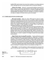
10-1
Introduction 681
10-2 Tuning Rules for PID Controllers 682
10-3 Computational Approach to Obtain Optimal Sets of Parameter
Values 692
104

Modifications of PID Control Schemes 700
10-5 Two-Degrees-of-Freedom Control 703
10-6 Zero-Placement Approach to Improve Response
Characteristics 705
Example Problems and Solutions 724
Problems 745
Chapter
1 1
Analysis of Control Systems in State Space
11-1
Introduction 752
11-2 State-Space Representations of Transfer-Function Systems 753
11-3 Transformation of System Models with
MATLAB 760
11-4
Solving the Time-Invariant State Equation 764
11-5 Some Useful Results in Vector-Matrix Analysis 772
11-6 Controllability 779
11-7 Observability 786
Example Problems and Solutions 792
Problems 824
Contents
Chapter
12
Design of Control Systems in State Space
12-1 Introduction 826
12-2 Pole Placement 827
12-3 Solving Pole-Placement Problems with
MATLAB
839

12-4 Design of Servo Systems 843
12-5 State Observers 855
12-6 Design of Regulator Systems with Observers 882
12-7 Design of Control Systems with Observers 890
12-8 Quadratic Optimal Regulator Systems 897
Example Problems and Solutions 910
Problems 948
References
Index
Contents
Preface
This book presents a comprehensive treatment of the analysis and design of control sys-
tems. It is written at the level of the senior engineering (mechanical, electrical, aero-
space, and chemical) student and is intended to be used as a text for the first course in
control systems. The prerequisite on the part of the reader is that he or she has had
introductory courses on differential equations, vector-matrix analysis, circuit analysis,
and mechanics.
The main revision made in the fourth edition of the text is to present two-degrees-
of-freedom control systems to design high performance control systems such that
steady-
state errors in following step, ramp, and acceleration inputs become zero. Also, newly
presented is the computational
(MATLAB) approach to determine the pole-zero loca-
tions of the controller to obtain the desired transient response characteristics such that
the maximum overshoot and settling time in the step response be within the specified
values. These subjects are discussed in Chapter 10. Also, Chapter
5
(primarily transient
response analysis) and Chapter 12 (primarily pole placement and observer design) are
expanded using

MATLAB. Many new solved problems are added to these chapters so
that the reader will have a good understanding of the
MATLAB
approach to the analy-
sis and design of control systems. Throughout the book computational problems are
solved with
MATLAB.
This text is organized into
12
chapters.The outline of the book is as follows. Chapter
1
presents an introduction to control systems. Chapter 2 deals with Laplace transforms of
commonly encountered time functions and some of the useful theorems on
Laplace
transforms.
(If
the students have an adequate background on Laplace transforms, this
chapter may be skipped.) Chapter
3
treats mathematical modeling of dynamic systems
(mostly mechanical, electrical, and electronic systems) and develops transfer function
models and state-space models. This chapter also introduces signal flow graphs. Discus-
sions of a linearization technique for nonlinear mathematical models are included in
this chapter.
Chapter
4
presents mathematical modeling of fluid systems (such as liquid-level sys-
tems, pneumatic systems, and hydraulic systems) and thermal systems. Chapter
5
treats

transient response analyses of dynamic systems to step, ramp, and impulse inputs.
MATLAB is extensively used for transient response analysis. Routh's stability criteri-
on is presented in this chapter for the stability analysis of higher order systems.
Steady-
state error analysis of unity-feedback control systems is also presented in this chapter.
Chapter
6
treats the root-locus analysis of control systems. Plotting root loci with
MATLAB is discussed in detail. In this chapter root-locus analyses of positive-feedback
systems, conditionally stable systems, and systems with transport lag are included. Chap-
ter
7
presents the design of lead, lag, and lag-lead compensators with the root-locus
method. Both series and parallel compensation techniques are discussed.
Chapter
8
presents basic materials on frequency-response analysis. Bode diagrams,
polar plots, the Nyquist stability criterion, and closed-loop frequency response are dis-
cussed including the
MATLAB approach to obtain frequency response plots. Chapter
9
treats the design and compensation techniques using frequency-response methods.
Specifically, the Bode diagram approach to the design of lead, lag, and lag-lead com-
pensators is discussed in detail.
Chapter 10 first deals with the basic and modified PID controls and then presents
computational
(MATLAB) approach to obtain optimal choices of parameter values
of controllers to satisfy requirements on step response characteristics. Next, it presents
two-degrees-of-freedom control systems. The chapter concludes with the design of
high performance control systems that will follow a step, ramp, or acceleration input

without steady-state error. The zero-placement method is used to accomplish such
performance.
Chapter
11
presents a basic analysis of control systems in state space. Concepts of
controllability and observability are given here. This chapter discusses the transforma-
tion of system models (from transfer-function model to state-space model, and vice
versa) with
MATLAB. Chapter 12 begins with the pole placement design technique,
followed by the design of state observers. Both full-order and minimum-order state ob-
servers are treated. Then, designs of type
1
servo systems are discussed in detail. In-
cluded in this chapter are the design of regulator systems with observers and design of
control systems with observers. Finally, this chapter concludes with discussions of quad-
ratic optimal regulator systems.
'
In this book, the basic concepts involved are emphasized and highly mathematical
arguments are carefully avoided in the presentation of the materials. Mathematical
proofs are provided when they contribute to the understanding of the subjects pre-
sented. All the material has been organized toward a gradual development of control
theory.
Throughout the book, carefully chosen examples are presented at strategic points so
that the reader will have a clear understanding of the subject matter discussed. In addi-
tion, a number of solved problems (A-problems) are provided at the end of each chap-
ter, except Chapter
1.
These solved problems constitute an integral part of the text.
Therefore, it is suggested that the reader study all these problems carefully to obtain a
deeper understanding of the topics discussed. In addition, many problems (without so-

lutions) of various degrees of difficulty are provided
(B-problems).These problems may
be used as homework or quiz purposes. An instructor using this text can obtain a com-
plete solutions manual (for B-problems) from the publisher.
Most of the materials including solved and unsolved problems presented in this book
have been class tested in senior level courses on control systems at the University of
Minnesota.
If this book is used as a text for a quarter course (with 40 lecture hours), most of the
materials in the first 10 chapters (except perhaps Chapter
4)
may be covered. [The first
nine chapters cover all basic materials of control systems normally required in a first
course on control systems. Many students enjoy studying computational
(MATLAB)
approach to the design of control systems presented in Chapter 10. It is recommended
that Chapter 10 be included
in
any control courses.] If this book is used as a text for a
semester course (with
56
lecture hours), all or a good part of the book may be covered
with flexibility in skipping certain subjects. Because of the abundance of solved prob-
lems (A-problems) that might answer many possible questions that the reader might
have, this book can also serve as a self-study book for practicing engineers who wish to
study basic control theory.
I would like to express my sincere appreciation to Professors
Athimoottil
V.
Mathew
(Rochester Institute of Technology), Richard Gordon (University of Mississippi), Guy

Beale (George Mason University), and Donald
T.
Ward (Texas A
&
M University), who
made valuable suggestions at the early stage of the revision process, and anonymous re-
viewers who made many constructive comments. Appreciation is also due to my former
students, who solved many of the A-problems and B-problems included in this book.
Katsuhiko
Ogata
Preface
Introduction
to Control Systems
Automatic control has played a vital role in the advance of engineering and science. In
addition to its extreme importance
$
space-vehicle systems, missile-guidance systems,
robotic systems, and the like, automatic control has become an important and integral
part of modern manufacturing and industrial processes. For example, automatic control
is essential in the numerical control of machine tools in the manufacturing industries,
in the design of autopilot systems in the aerospace industries, and in the design of cars
and trucks in the automobile industries. It is also essential in such industrial operations
as controlling pressure, temperature, humidity, viscosity, and flow in the process
industries.
Since advances in the theory
and practice of automatic control provide the means for
attaining optimal performance of dynamic systems, improving productivity, relieving
the drudgery of many routine repetitive manual operations, and more, most engineers
and scientists must now have a good understanding of this field.

Historical
Review.
The first significant work in automatic control was James Watt's
centrifugal governor for the speed control of a steam engine in the eighteenth century.
Other significant works in the early stages of development of control theory were due
to Minorsky, Hazen, and Nyquist, among many others. In 1922,
Minorsky worked on
automatic controllers for steering ships and showed how stability could be determined
from the differential equations describing the system. In
1932,Nyquist developed a rel-
atively simple procedure for determining the stability of closed-loop systems on the
basis of open-loop response to steady-state sinusoidal inputs. In 1934, Hazen, who in-
troduced the term servomechanisms for position control systems, discussed the design
of relay servomechanisms capable of closely following a changing input.
During the decade of the
1940s, frequency-response methods (especially the Bode
diagram methods due to Bode) made it possible for engineers to design linear closed-
loop control systems that satisfied performance requirements. From the end of the 1940s
to the early
1950s, the root-locus method due to Evans was fully developed.
The frequency-response and root-locus methods, which are the core of classical con-
trol theory, lead to systems that are stable and satisfy a set of more or less arbitrary per-
formance requirements. Such systems are, in general, acceptable but not optimal in any
meaningful sense. Since the late
1950s, the emphasis in control design problems has been
shifted from the design of one of many systems that work to the design of one optimal
system in some meaningful sense.
As modern plants with many inputs and outputs become more and more complex,
the description of a modern control system requires a large number of equations. Clas-
sical control theory, which deals only with single-input-single-output systems, becomes

powerless for multiple-input-multiple-output systems. Since about 1960, because the
availability of digital computers made possible time-domain analysis of complex sys-
tems, modern control theory, based on time-domain analysis and synthesis using state
variables, has been developed to cope with the increased complexity of modern plants
and the stringent requirements on accuracy, weight, and cost in military, space, and in-
dustrial applications.
During the years from 1960 to 1980, optimal control of both deterministic and sto-
chastic systems, as well as adaptive and learning control of complex systems, were fully
investigated. From 1980 to the present, developments in modern control theory cen-
tered around robust control,
H,
control, and associated topics.
Now that digital computers have become cheaper and more compact, they are used
as
integral parts of control systems. Recent applications of modern control theory include
such nonengineering systems as biological, biomedical, economic, and socioeconomic
systems.
Definitions.
Before we can discuss control systems, some basic terminologies must
be defined.
Controlled Variable and Manipulated Variable.
The
controlled
variable is
the quantity or condition that is measured and controlled. The
manipulated
variable
is the quantity or condition that is varied by the controller so as to affect the value of
the controlled variable. Normally, the controlled variable is the output of the system.
Control

means measuring the value of the controlled variable of the system and ap-
plying the manipulated variable to the system to correct or limit deviation of the meas-
ured value from a desired value.
In studying control engineering, we need to define additional terms that are neces-
sary to describe control systems.
Plants.
A
plant may be a piece of equipment, perhaps just a set of machine parts
functioning together, the purpose of which is to perform a particular operation. In this
book, we shall call any physical object to be controlled (such as a mechanical device, a
heating furnace, a chemical reactor, or a spacecraft) a plant.
Chapter
1
/
Introduction to Control Systems
Processes.
The Merriam-Webster Dictionary defines a process to be a natural, pro-
gressively continuing operation or development marked by a series of gradual changes
that succeed one another in a relatively fixed way and lead toward a particular result or
end; or an artificial or voluntary, progressively continuing operation that consists of a se-
ries of controlled actions or movements systematically directed toward a particular re-
sult or end. In this book we shall call any operation to be controlled aprocess. Examples
are chemical, economic, and biological processes.
Systems.
A
system is a combination of components that act together and perform
a certain objective.
A
system is not limited to physical ones. The concept of the system
can be applied to abstract, dynamic phenomena such as those encountered in econom-

ics. The word system should, therefore, be interpreted to imply physical, biological, eco-
nomic, and the like, systems.
Disturbances.
A
disturbance is a signal that tends to adversely affect the value of
the output of a system.
If
a disturbance is generated within the system, it is called inter-
nal,
while an external disturbance is generated outside the system and is an input.
Feedback Control.
Feedback control refers to an operation that, in the presence
of disturbances, tends to reduce the difference between the output of a system and some
reference input and does so on the basis of this difference. Here only unpredictable dis-
turbances are so specified, since predictable or known disturbances can always be com-
pensated for within the system.
1-2
WWPLES OF CONTROL SYSTEMS
In this section we shall present several examples of control systems.
Speed Control System.
The basic principle of a Watt's speed governor for an
engine is illustrated in the schematic diagram of Figure
l-1.The amount of fuel admitted
Figure
1-11
Speed
control
Control
system.
valve

Section
1-2
/
Examples of Control Systems
'Thermometer
/"
Figure
1-2
Temperature
(
system.
to the engine is adjusted according to the difference between the desired and the actual
engine speeds.
The sequence of actions may be stated as
follows:The speed governor is adjusted such
that, at the desired speed, no pressured oil will flow into either side of the power cylin-
der.
If
the actual speed drops below the desired value due to disturbance, then the de-
crease in the centrifugal force of the speed governor causes the control valve to move
downward, supplying more fuel, and the speed of the engine increases until the desired
value is reached. On the other hand, if the speed of the engine increases above the de-
sired value, then the increase in the centrifugal force of the governor causes the control
valve to move upward. This decreases the supply of fuel, and the speed of the engine
decreases until the desired value is reached.
In
this speed control system, the plant (controlled system) is the engine and the con-
trolled variable is the speed of the engine. The difference between the desired speed
and the actual speed is the error
signal.The control signal (the amount of fuel) to be ap-

plied to the plant (engine) is the actuating signal. The external input to disturb the con-
trolled variable is the disturbance. An unexpected change in the load is a disturbance.
Temperature Control System.
Figure
1-2
shows a schematic diagram of tem-
perature control of an electric furnace. The temperature in the electric furnace is meas-
ured by a thermometer, which is an analog device. The analog temperature is converted
to a digital temperature
by
an
ND
converter. The digital temperature is fed to a con-
troller through an
interface.This digital temperature is compared with the programmed
input temperature, and if there is any discrepancy (error), the controller sends out a sig-
nal to the heater, through an interface, amplifier, and relay, to bring the furnace tem-
perature to a desired value.
EXAMPLE
1-1
Consider the temperature control of the passenger compartment of
a
car.The desired temperature
(converted to a voltage)
is
the input to the controller. The actual temperature of the passenger
compartment must be converted to a voltage through
a
sensor and fed back
to

the controller for
comparison
with
the input.
Figure
1-3
is
a
functional block diagram of temperature control of the passenger compartment
of
a
car.
Note that the ambient temperature and radiation heat transfer from the sun, which are
not
constant
while
the car is driven, act as disturbances.
4
Chapter
1
/
Introduction to Control
Systems
Ambient
Sun temperature
Sensor
s
Radiation
heat sensor
Y

Y
t
t
Passenger
Desired
compartment
temperature Heater or
temperature
i
Controller
-
air
Passenger
-
(Input) conditioner
-
compartment (Output)
Figure
G.3
A
The temperature of the passenger compartment differs considerably depending on the place
where it is measured. Instead of using multiple sensors for temperature measurement and
averaging the measured values, it is economical to install a small suction blower at the place where
passengers normally sense the temperature. The temperature of the air from the suction blower
is an indication of the passenger compartment temperature and is considered the output of the
system.
The controller receives the input signal, output signal, and signals from sensors from
disturbance sources. The controller sends out an optimal control signal to the air conditioner or
heater to control the amount of cooling air or warm air so that the passenger compartment
temperature is about the desired temperature.

Temperature control
of passenger
compartment
Business Systems.
A
business system may consist of many groups. Each task
assigned to a group will represent a dynamic element of the system. Feedback methods
of reporting the accomplishments of each group must be established in such a system for
proper
operation.'~he cross-coupling between functional groups must be made a mini-
mum in order to reduce undesirable delay times in the system. The smaller this cross-
coupling, the smoother the flow of work signals and materials will be.
A
business system is a closed-loop system.
A
good design will reduce the manageri-
al
control required. Note that disturbances in this system are the lack of personnel or ma-
terials, interruption of communication, human errors, and the like.
The establishment of a well-founded estimating system based on statistics is manda-
tory to proper management. Note that it is a well-known fact that the performance of
such
a
system can be improved by the use of lead time,
or
anticipation.
To apply control theory to improve the performance of such a system, we must rep-
resent the dynamic characteristic of the component groups of the system by a relative-
ly simple set of equations.
Although it is certainly a difficult problem to derive mathematical representations

of the component groups, the application of optimization techniques to business sys-
tems significantly improves the performance of the business system.
-
Section
1-2
/
Examples of Control Systems
5
of a car.
Figure
1-4
Block diagram of an engineering organizational system.
Required
EXAMPLE
1-2
An engineering organizational system is composed of major groups such as management, research
and development, preliminary design, experiments, product design and drafting, fabrication and
assembling, and
testing.These groups are interconnected to make up the whole operation.
Such a system may be analyzed by reducing it to the most elementary set of components
product
+
IIGLG~~~I~
LII~L
L~II
~IOVIUG
LI~G
aIialyLical uetall loquircu anu
uy
IepIesenilIlg Lne uynarrilc cnar-

acteristics of each component by a set of simple equations. (The dynamic performance of such a
system may be determined from the relation between progressive accomplishment and time.)
Draw a functional block diagram showing an engineering organizational system.
A functional block diagram can be drawn by using blocks to represent the functional activi-
ties and interconnecting signal lines to represent the information or product output of the system
operation.
A
possible block diagram is shown in Figure
14.
1-3
CLOSED-LOOP CONTROL VERSUS OPEN-LOOP CONTROL
h
t
Management
Feedback Control Systems.
A
system that maintains a prescribed relationship
between the output and the reference input by comparing them and using the difference
as a means of control is called a
feedback control system.
An example would be a room-
temperature control system. By measuring the actual room temperature and comparing
;t Ath thn mfnmnon tnmnor~t~~ra /Ancl;mA tomnor~t~~ro\ tho thermnrt~t tnmr the hest.
1L WlLll Lllb
1
blLlb1IC.b LbIIIYbL LILUI
b
\UbJII
VU
LbIIIYVI ULUIb,, CIIb LII.21 IIIVLICUL

L"111.3
CllU
1IVUL
ing or cooling equipment on or off in such a way as to ensure that the room tempera-
ture remains at a comfortable level regardless of outside conditions.
Feedback control systems are not limited to engineering but can be found in various
nonengineering fields as well. The human body, for instance, is a highly advanced feed-
back control system. Both body temperature and blood pressure are kept constant by
means of physiological feedback. In fact, feedback performs a vital function: It makes
the human body relatively insensitive to external disturbances, thus enabling it to func-
tion properly in a changing environment.
-+
Closed-Loop Control Systems.
Feedback control systems are often referred to
as
closed-loop control
systems. In practice, the terms feedback control and closed-loop
control are used interchangeably. In a closed-loop control system the actuating error
signal, which is the difference between the input signal and the feedback signal (which
may be the output signal itself or a function of the output signal and its derivatives
and/or integrals), is fed to the controller so as to reduce the error and bring the output
of the system to a desired
value.The term closed-loop control always implies the use of
feedback control action in order to reduce system error.
Research
and
development
Open-Loop Control Systems.
Those systems in which the output has no effect
on the control action are called

open-loop control systems.
In other words, in an open-
-
Chapter
1
/
Introduction to Control Systems
Preliminary
design
Experiments
Product
design and
drafting
v
-+
Fabrication
and
assembl~ng
Product
-+
.
Testing
*
loop control system the output is neither measured nor fed back for comparison with the
input. One practical example is a washing machine. Soaking, washing, and rinsing in the
washer operate on a time basis. The machine does not measure the output signal, that
is, the cleanliness of the clothes.
In any open-loop control system the output is not compared with the reference input.
Thus, to each reference input there corresponds a fixed operating condition; as a result,
the accuracy of the system depends on calibration. In the presence of disturbances, an

open-loop control system will not perform the desired task. Open-loop control can be
used, in practice, only if the relationship between the input and output is known and if
there are neither internal nor external disturbances. Clearly, such systems are not feed-
back control systems. Note that any control system that operates on a time basis is open
loop. For instance, traffic control by means of signals operated on a time basis is another
example.of open-loop control.
Closed-Loop versus Open-Loop Control Systems.
An advantage of the closed-
loop control system is the fact that the use of feedback makes the system response rel-
atively insensitive to external disturbances and internal variations in system parameters.
It
is thus possible to use relatively inaccurate and inexpensive components to obtain
the accurate control of a given plant, whereas doing so is impossible in the open-loop
case.
From the point of view of stability, the open-loop control system is easier to build be-
cause system stability is not a major problem. On the other hand, stability is a major
problem in the closed-loop control system, which may tend to overcorrect errors and
thereby can cause oscillations of constant or changing amplitude.
It should be emphasized that for systems in which the inputs are known ahead of time
and in which there are no disturbances it is advisable to use open-loop control. Closed-
loop control systems have advantages only when unpredictable disturbances
and/or
un-
predictable variations in system components are present. Note that the output power
rating partially determines the cost, weight, and size of a control
system.The number of
components used in a closed-loop control system is more than that for a corresponding
open-loop control system. Thus, the closed-loop control system is generally higher in
cost and power. To decrease the required power of a system, open-loop control may be
used where applicable.

A
proper combination of open-loop and closed-loop controls is
usually less expensive and will give satisfactory overall system performance.
EXAMPLE
1-3
Most analyses and designs of control systems presented in this book are concerned with closed-
loop control systems. Under certain circumstances (such as where no disturbances exist or the
output is hard to measure) open-loop control systems may be
desired.Therefore, it is worthwhile
to summarize the advantages and disadvantages of using open-loop control systems.
The major advantages of open-loop control systems are as follows:
1.
Simple construction and ease of maintenance.
2.
Less expensive than a corresponding closed-loop system.
3.
There is no stability problem.
4.
Convenient when output is hard to measure or measuring the output precisely is economi-
cally not feasible. (For example, in the washer
system,it would be quite expensive to provide
a device to measure the quality of the washer's output, cleanliness of the clothes.)
Section
1-3
/
Closed-Loop Control versus Open-Loop Control
7
The major disadvantages of open-loop control systems are as follows:
1.
Disturbances and changes in calibration cause errors, and the output may be different from

what is desired.
2.
To maintain the required quality
in
the output, recalibration
is
necessary from time to time.
1-4
OUTLINE
OF
THE
BOOK
We briefly describe here the organization and contents of the book.
Chapter
1
has given introductory materials on control systems. Chapter
2
presents
basic
Laplace transform theory necessary for understanding the control theory pre-
sented in this book. Chapter
3
deals with mathematical modeling of dynamic systems in
terms of transfer functions and state-space equations. It discusses mathematical model-
ing of mechanical systems and electrical and electronic systems. This chapter also in-
cludes the signal flow graphs and linearization of nonlinear mathematical models.
Chapter
4
treats mathematical modeling of liquid-level systems, pneumatic systems, hy-
draulic systems, and thermal systems. Chapter

5
treats transient-response analyses of
first-,and second-order systems as well as higher-order systems. Detailed discussions of
transient-response analysis with
MATLAB are presented. Routh's stability criterion
and steady-state errors in unity-feedback control systems are also presented in this
chapter.
Chapter
6
gives a root-locus analysis of control systems. General rules for constructing
root loci are presented. Detailed discussions for plotting root loci with
MATLAB are in-
cluded. Chapter
7
deals with the design of control systems via the root-locus method.
Specifically, root-locus approaches to the design of lead compensators, lag compensators,
and lag-lead compensators are discussed in detail. Chapter
8
gives the frequency-
response analysis of control systems. Bode diagrams, polar plots, Nyquist stability crite-
rion, and closed-loop frequency response are discussed. Chapter
9
treats control systems
design via the frequency-response approach. Here Bode diagrams are used to design
lead compensators, lag compensators, and lag-lead compensators. Chapter
10
discusses
the basic and modified PID controls. In this chapter two-degrees-of-freedom control
systems are introduced. We design high-performance control systems using two-degrees-
of-freedom configuration.

MATLAB is extensively used in the design of such systems.
Chapter
11
presents basic materials for the state-space analysis of control systems.
The solution of the time-invariant state equation is derived and concepts of controlla-
bility and observability are discussed. Chapter
12
treats the design of control systems in
state space. This chapter begins with the pole-placement problems, followed by the de-
sign of state observers, and the design of regulator systems with observers and control
systems with observers. Finally, quadratic optimal control is discussed.
Chapter
1
/
Introduction to Control Systems
The
Laplace
Transform
*
2-1
INTRODUCTION
The Laplace transform method is an ope~ational method that can be used advanta-
geously for solving linear differential equations. By use of
Laplace transforms, we can
convert many common functions, such as sinusoidal functions, damped sinusoidal func-
tions, and exponential functions, into algebraic functions of a complex variable
s.
Op-
erations such as differentiation and integration can be replaced by algebraic operations
in the complex

plane.Thus, a linear differential equation can be transformed into an al-
gebraic equation in a complex variable
s.
If the algebraic equation in
s
is solved for the
dependent variable, then the solution of the differential equation (the inverse
Laplace
transform of the dependent variable) may be found by use of a Laplace transform table
or by use of the partial-fraction expansion technique, which is presented in Section 2-5
and
2-6.
An advantage of the Laplace transform method is that it allows the use of graphical
techniques for predicting the system performance without actually solving system dif-
ferential equations. Another advantage of the
Laplace transform method is that, when
we solve the differential equation, both the transient component and steady-state com-
ponent of the solution can be obtained simultaneously.
Outline
of
the Chapter.
Section
2-1
presents introductory remarks. Section 2-2
briefly reviews complex variables and complex functions. Section 2-3 derives
Laplace
*This chapter may be skipped
if
the student is already familiar with Laplace transforms.
transforms of time functions that are frequently used in control engineering. Section

2-4
presents useful theorems of Laplace transforms, and Section
i-5
treats the inverse
Laplace transformation using the partial-fraction expansion of
B(s)/A(s),
where
A(s)
and
B(s)
are polynomials in
s.
Section
2-6
presents computational methods with
MAT-
LAB to obtain the partial-fraction expansion of
B(s)/A(s),
as well as the zeros and
poles of
B(s)/A(s).
Finally, Section
2-7
deals with solutions of linear time-invariant dif-
ferential equations by the
Laplace transform approach.
2-2
REVIEW
OF COMPLEX VARIABLES
AND COMPLEX FUNCTIONS

Before we present the Laplace transformation, we shall review the complex variable
and complex function. We shall also review Euler's theorem, which relates the
sinu-
soidal functions to exponential'functions.
Complex Variable.
A complex number has a real part and an imaginary part, both
of which are constant. If the real part
and/or imaginary part are variables, a complex
quantity is called a
complex variable.
In the Laplace transformation we use the notation
s
as a complex variable; that is,
where
a
is the real part and
w
is the imaginary part.
Complex Function.
A complex function
G(s),
a function of
s,
has a real part and
an imaginary part or
G(s)
=
Gx
+
jG,

where
Gx
and
G,
are real quantities. The magnitude of
G(s)
is
I/-,
and the
angle
13
of
G(s)
is
tan-'(~,/~,).
The angle is measured counterclockwise from the pos-
itive real axis. The complex conjugate of
G(s)
is
G(s)
=
G,
-
jG,.
Complex functions commonly encountered in linear control systems analysis are
single-valued functions of
s
and are uniquely determihed for
a
given value of

s.
A complex function
G(s)
is said to be
analytic
in a region if
G(s)
and all its deriva-
tives exist in that region. The derivative of an analytic function
G(s)
is given by
d
.
G(s
+
As)
-
G(s)
-G(s)
=
lim
AG
=
lim

d~
AS+~
AS
As+O
As

Since
As
=
Aa
+
jAw, As
can approach zero along an infinite number of different
paths. It can be shown, but is stated without a proof here, that if the derivatives taken
along two particular paths, that is,
As
=
Au
and
As
=
jAw,
are equal, then the deriva-
tive is unique for any other path
As
=
Aa
+
jAw
and so the derivative exists.
For a particular path
As
=
Au
(which means that the path is parallel to the real
axis).

Chapter
2
/
The Laplace Transform
For another particular path As
=
jAw (which means that the path is parallel to the
imaginary axis).
d
dGx
,
AGy
-
G(s)
=
lim
ds
-j-+
If
these two values of the derivative are equal,
or if the following two conditions
are satisfied, then the derivative
dG (s)/ ds is uniquely determined.These two conditions
are known as the Cauchy-Riemann conditions. If these conditions are satisfied, the func-
tion
G(s) is analytic.
As an example, consider the following
G(s):
Then
where

a
+
1
-w
Gx
=
and Gy
=
(a
+
+
w2
(a
+
+
w2
It can be seen that, except at s
=
-1
(that is,
a
=
-1,
w
=
0),
G(s) satisfies the
Cauchy-Riemann conditions:
dGx aGy w2
-

(a
+
1)2

-

-
dff
[(u
+
1)2
+
w2I2
Hence G(s)
=
l/(s
+
1) is analytic in the entire s plane except at s
=
-1.The deriva-
tive
dG (s)/ ds, except at s
=
1,
is found to be
Note that the derivative of an analytic function can be obtained simply by differentiat-
ing
G(s) with respect to
s.
In this example,

Section
2-1
/
Review of Complex Variables and Complex Functions
Points in the
s
plane at which the function
G(s)
is analytic are called ordinary points,
while points in the
s
plane at which the function
G(s)
is not analytic are called singular
points. Singular points at which the function
G(s)
or its derivatives approach infinity
are
calledpoles. Singular points at which the function
G(s)
equals zero are called zeros.
If
G(s)
approaches infinity as
s
approaches -p and if the function
has a finite, nonzero value at
s
=
-p, then

s
=
-p
is called a pole of order
n.
If n
=
1,
the pole is called a simple pole. If
n
=
2,3,.
. .
,
the pole is called a second-order pole, a
third-order pole, and so on.
To illustrate, consider the complex function
G(s)
has zeros at
s
=
-2,
s
=
-10,
simple poles at
s
=
0, s
=

-1, s
=
-5,
and a double
pole (multiple pole of order 2) at
s
=
-15.
Note that
G(s)
becomes zero at
s
=
co.
Since
for large values of
s
G(s)
possesses a triple zero (multiple zero of order
3)
at
s
=
co.
If points at infinity are
included,
G(s)
has the same number of poles as zeros.To summarize,
G(s)
has five zeros

(s
=
-2,
s
=
-10,
s
=
co,
s
=
co, s
=
co)
and five poles
(s
=
0,
s
=
-1,
s
=
-5,
s
=
-15, s
=
-15).
Euler's

Theorem.
The power series expansions of cos
0
and sin
0
are, respectively,
And so
Since
we see that
cos
8
+
j
sin
0
=
eis
This is known as Euler's
theorem.
Chapter
2
/
The Laplace Transform