enhanced oil recovery - larry w. lake
Bạn đang xem bản rút gọn của tài liệu. Xem và tải ngay bản đầy đủ của tài liệu tại đây (10.46 MB, 414 trang )
1
1
Defining Enhanced Oil
Recovery
Enhanced oil recovery (EOR) is oil recovery by the injection of materials not
normally present in the reservoir. This definition covers all modes of oil recovery
processes (drive, push-pull, and well treatments) and most oil recovery agents.
Enhanced oil recovery technologies are also being used for in-situ extraction of
organic pollutants from permeable media. In these applications, the extraction is
referred to as cleanup or remediation, and the hydrocarbon as product. Various
sections of this text will discuss remediation technologies specifically, although we
will mainly discuss petroleum reservoirs. The text will also describe the application
of EOR technology to carbon dioxide storage where appropriate.
The definition does not restrict EOR to a particular phase (primary,
secondary, or tertiary) in the producing life of a reservoir. Primary recovery is oil
recovery by natural drive mechanisms: solution gas, water influx, and gas cap drives,
or gravity drainage. Figure 1-1 illustrates. Secondary recovery refers to techniques,
such as gas or water injection, whose purpose is mainly to raise or maintain reservoir
pressure. Tertiary recovery is any technique applied after secondary recovery. Nearly
all EOR processes have been at least field tested as secondary displacements. Many
thermal methods are commercial in both primary and secondary modes. Much
interest has been focused on tertiary EOR, but the definition given here is not so
restricted. The definition does exclude waterflooding but is intended to exclude
all pressure maintenance processes. The distinction between pressure maintenance
2
and displacement is not clear, since some displacement occurs in all pressure
maintenance processes. Moreover, agents such as methane in a high-pressure gas
drive, or carbon dioxide in a reservoir with substantial native CO
2
, do not satisfy the
definition, yet both are clearly EOR processes. The same can be said of CO
2
storage.
Usually the EOR cases that fall outside the definition are clearly classified by the
intent of the process.
In the last decade, improved oil recovery (IOR) has been used
interchangeably with EOR or even in place of it. Although there is no formal
definition, IOR typically refers to any process or practice that improves oil recovery
(Stosur et al., 2003). IOR therefore includes EOR processes but can also include
other practices such as waterflooding, pressure maintenance, infill drilling, and
horizontal wells.
Conventional
Recovery
Enhanced
Recovery
Other
Chemical
Solvent
Thermal
Pressure Maintenance
Water/Gas Reinjection
Artificial Lift
Pump - Gas Lift
Waterflood
Natural Flow
Tertiary
Recovery
Secondary
Recovery
Primary
Recovery
Conventional
Recovery
Enhanced
Recovery
OtherOther
ChemicalChemical
SolventSolvent
ThermalThermal
Pressure Maintenance
Water/Gas Reinjection
Pressure Maintenance
Water/Gas Reinjection
Artificial Lift
Pump - Gas Lift
Artificial Lift
Pump - Gas Lift
WaterfloodWaterflood
Natural FlowNatural Flow
Tertiary
Recovery
Secondary
Recovery
Primary
Recovery
Tertiary
Recovery
Secondary
Recovery
Primary
Recovery
Figure 1-1. Oil recovery classifications (adapted from the Oil and Gas Journal
biennial surveys).
1-1 EOR INTRODUCTION
The EOR Target
We are interested in EOR because of the amount of oil to which it is potentially
applicable. This EOR target oil is the amount unrecoverable by conventional means
(Fig. 1-1). A large body of statistics shows that conventional ultimate oil recovery
(the percentage of the original oil in place at the time for which further conventional
3
recovery becomes uneconomic) is about 35%. This means for example that a field
that originally contained 1 billion barrels will leave behind 650,000 barrels at the end
of its conventional life. Considering all of the reservoirs in the U.S., this value is
much larger than targets from exploration or increased drilling.
The ultimate recovery is shown in Fig. 1-2. This figure also shows that there
is enormous variability in ultimate recovery within a geographic region, which is why
we cannot target reservoirs with EOR by region. Reservoirs that have an
exceptionally large conventional recovery are not good tertiary EOR candidates.
Figure 1-2 shows also that the median ultimate recovery is the same for most regions,
a fact no doubt bolstered by the large variability within each region.
0
20
40
60
80
100
Middle East CIS LatAm Africa Far East Europe Austral Asia US
Ultimate Recovery Efficiency, %
Figure 1-2. Box plots of ultimate oil recovery efficiency. 75% of the ultimate
recoveries in a region fall within the vertical boxes; the median recovery is the
horizontal line in the box; the vertical lines give the range. Ultimate recovery is
highly variable, but the median is about the same everywhere (from Laherre, 2001).
1-2 THE NEED FOR EOR
Enhanced oil recovery is one of the technologies needed to maintain reserves.
Reserves
4
Reserves are petroleum (crude and condensate) recoverable from known reservoirs
under prevailing economics and technology. They are given by the following
material balance equation:
Production
Present Past Additions
from
reserves reserves to reserves
reserves
⎛⎞
⎛⎞⎛⎞⎛ ⎞
⎜⎟
=+ −
⎜⎟⎜⎟⎜ ⎟
⎜⎟
⎝⎠⎝⎠⎝ ⎠
⎜⎟
⎝⎠
There are actually several categories of reservoirs (proven, etc.) which distinctions
are very important to economic evaluation (Rose, 2001; Cronquist, 2001). Clearly,
reserves can change with time because the last two terms on the right do change with
time. It is in the best interests of producers to maintain reserves constant with time,
or even to have them increase.
Adding to Reserves
The four categories of adding to reserves are
1.
Discovering new fields
2.
Discovering new reservoirs
3.
Extending reservoirs in known fields
4.
Redefining reserves because of changes in economics of extraction
technology
We discuss category 4 in the remainder of this text. Here we substantiate its
importance by briefly discussing categories 1 to 3.
Reserves in categories 1 to 3 are added through drilling, historically the most
important way to add reserves. Given the 2% annual increase in world-wide
consumption and the already large consumption rate, it has become evident that
reserves can be maintained constant only by discovering large reservoirs.
But the discovery rate of large fields is declining. More importantly, the
discovery rate no longer depends strongly on the drilling rate. Equally important,
drilling requires a substantial capital investment even after a field is discovered. By
contrast, the majority of the capital investment for EOR has already been made (if
previous wells can be used). The location of the target field is known (no need to
explore), and targets tend to be close to existing markets.
Enhanced oil recovery is actually a competitor with conventional oil
recovery because most producers have assets or access to assets in all of the Fig. 1-1
categories. The competition then is joined largely on the basis of economics in
addition to reserve replacement. At the present, many EOR technologies are
competitive with drilling-based reserve additions. The key to economic
competitiveness is how much oil can be recovered with EOR, a topic to which we
next turn.
5
1-3 INCREMENTAL OIL
Defintion
A universal technical measure of the success of an EOR project is the amount of
incremental oil recovered. Figure 1-3 defines incremental oil. Imagine a field,
reservoir, or well whose oil rate is declining as from
A to B. At B, an EOR project is
initiated and, if successful, the rate should show a deviation from the projected
decline at some time after
B. Incremental oil is the difference between what was
actually recovered,
B to D, and what would have been recovered had the process not
been initiated,
B to C. Since areas under rate-time curves are amounts, this is the
shaded region in Fig. 1-3.
Figure 1-3. Incremental oil recovery from typical
EOR response (from Prats, 1982)
6
As simple as the concept in Fig. 1-3 is, EOR is difficult to determine in
practice. There are several reasons for this.
1. Combined (comingled) production from EOR and nonEOR wells. Such
production makes it difficult to allocate the EOR-produced oil to the EOR
project. Comingling occurs when, as is usually the case, the EOR project is
phased into a field undergoing other types of recovery.
2. Oil from other sources. Usually the EOR project has experienced substantial
well cleanup or other improvements before startup. The oil produced as a
result of such treatment is not easily differentiated from the EOR oil.
3.
Inaccurate estimate of hypothetical decline. The curve from B to C in Fig. 1-
3 must be accurately estimated. But since it did not occur, there is no way of
assessing this accuracy.
Ways to infer incremental oil recovery from production data range from highly
sophisticated numerical models to graphical procedures. One of the latter, based on
decine curve analysis, is covered in the next section.
Estimating Incremental Oil Recovery Through Decline Curves
Decline curve analysis can be applied to virtually any hydrocarbon production
operation. The following is an abstraction of the practice as it applies to EOR. See
Walsh and Lake (2003) for more discussion. The objective is to derive relations
between oil rate and time, and then between cumulative production and rate.
The oil rate
q changes with time t in a manner that defines a decline rate D
according to
1 dq
D
qdt
=
− 1.3-1
The rate has units of (or [=]) amount or volume per time and
D [=]1/time. Time is in
units of days, months, or even years consistent with the units of
q. D itself can be a
function of rate, but we take it to be constant. Integrating Eq.
1.3-1 gives
D
t
i
qqe
−
= 1.3-2
where
q
i
is the initial rate or q evaluated at t = 0. Equation 1.3-2 suggests a
semilogarithmic relationship between rate and time as illustrated in Fig. 1-3.
Exponential decline is the most common type of analysis employed.
7
lo g (q)
q
i
q
EL
Decline
period
begins
Life
Slope =
-D
2.303
0
t
lo g (q)
q
i
q
EL
Decline
period
begins
Life
Slope =
-D
2.303
0
t
lo g (q)
q
i
q
EL
Decline
period
begins
Life
Slope =
-D
2.303
Slope =
-D
2.303
-D
2.303
0
t
Figure 1-3. Schematic of exponential decline on a rate-time plot.
Figure 1-3 schematically illustrates a set of data (points) which begin an
exponential decline at the ninth point where, by definition
t = 0. The solid line
represents the fit of the decline curve model to the data points.
q
i
is the rate given by
the model at
t=0, not necessarily the measured rate at this point. The slope of the
model is the negative of the decline rate divided by 2.303, since standard semilog
graphs are plots of base 10 rather than natural logarithms.
Because the model is a straight line, it can be extrapolated to some future
rate. If we let
q
EL
designate the economically limiting rate (simply the economic
limit
) of the project under consideration, then where the model extrapolation attains
q
EL
is an estimate of the project’s (of well’s, etc.) economic life. The economic limit
is a nominal measure of the rate at which the revenues become equal to operating
expenses plus overhead.
q
EL
can vary from a fraction to a few hundred barrels per
day depending on the operating conditions. It is also a function of the prevailing
economics: as oil price increases,
q
EL
decreases, an important factor in reserve
considerations.
The rate-time analysis is useful, but the rate-cumulative curve is more
helpful. The cumulative oil produced is given by
p
0
t
Nqd
ξ
ξ
ξ
=
=
=
∫
.
8
The definition in this equation is general and will be employed throughout the text,
but especially in Chap. 2. To derive a rate -cumulative expression, insert Eq. 1.3-1,
integrate, and identify the resulting terms with (again) Eq. 1.3-1. This gives
ip
qqDN=− 1.3-3
Equation
1.3-3 says that a plot of oil rate versus cumulative production should be a
straight line on linear coordinates. Figure 1-4 illustrates.
q
q
i
q
EL
Mobile oil
Slope = -D
0
N
p
Recoverable oil
q
q
i
q
EL
Mobile oil
Slope = -D
0
N
p
Recoverable oil
q
q
i
q
EL
Mobile oil
Slope = -D
0
N
p
Recoverable oil
Figure 1-4. Schematic of exponential decline on a rate-cumulative plot.
You should note that the cumulative oil points being plotted on the horizontal axis of
this figure are from the oil rate data, not the decline curve. It this were not so, there
would be no additional information in the rate-cumulative plot. Calculating
N
p
normally requires a numerical integration with something like the trapezoid rule.
Using model Eqs
1.3-2 and 1.3-3 to interpret a set of data as illustrated in
Figs. 1-3 and 1-4 is the essence of reservoir engineering practice, namely
1. Develop a model as we have done to arrive at Eqs.
1.3-2 and 1.3-3. Often the
model equations are far more complicated than these, but the method is the same
regardless of the model.
2. Fit the model to the data. Remember that the points in Figs. 1-3 and 1-4 are data.
The lines are the model.
3. With the model fit to the data (the model is now calibrated), extrapolate the model
to make predictions.
9
At the onset of the decline period, the data again start to follow a straight line
through which can be fit a linear model. In effect, what has occurred with this plot is
that we have replaced time on Fig. 1-3 with cumulative oil produced on Fig. 1-4, but
there is one very important distinction: both axes in Fig. 1-4 are now linear. This has
three important consequences.
1.
The slope of the model is now –D since no correction for log scales is
required.
2.
The origin of the model can be shifted in either direction by simple additions.
3.
The rate can now be extrapolated to zero.
Point 2 simply means that we can plot the cumulative oil produced for all
periods prior to the decline curve period (or for previous decline curve periods) on
the same rate-cumulative plot. Point 3 means that we can extrapolate the model to
find the total mobile oil (when the rate is zero) rather than just the recoverable oil
(when the rate is at the economic limit).
Rate-cumulative plots are simple yet informative tools for interpreting EOR
processes because they allow estimates of incremental oil recovery (IOR) by
distinguishing between recoverable and mobile oil. We illustrate how this comes
about through some idealized cases.
Figure 1-5 shows a rate-cumulative plot for a project having an exponential
decline just prior to and immediately after the initiation of an EOR process.
q
q
EL
Project begins
N
p
IOR
Incremental
mobile oil
q
q
EL
Project begins
N
p
IOR
Incremental
mobile oil
q
q
EL
Project begins
N
p
IOR
Incremental
mobile oil
Incremental
mobile oil
10
Figure 1-5. Schematic of exponential decline curve behavior on a rate-cumulative
plot. The EOR project produces both incremental oil (IOR), and increases the mobile
oil. The pre- and post-EOR decline rates are the same.
We have replaced the data points with the models only for ease of
presentation. Placing both periods on the same horizontal axis is permissible because
of the scaling arguments mentioned above. In this case, the EOR process did not
accelerate the production because the decline rates in both periods are the same;
however, the process did increase the amount of mobile oil, which in turn caused
some incremental oil production. In this case, the incremental recovery and mobile
oil are the same. Such idealized behavior would be characteristic of thermal,
micellar-polymer, and solvent processes.
q
q
EL
Project begins
N
p
IOR
q
q
EL
Project begins
N
p
IOR
q
q
EL
Project begins
N
p
IOR
Figure 1-6. Schematic of exponential decline curve behavior on a rate-cumulative
plot. The EOR project produces incremental oil at the indicated economic limit but
does not increase the mobile oil.
Figure 1-6 shows another extreme where production is only accelerated, the
pre- and post-EOR decline rates being different. Now the curves extrapolate to a
common mobile oil but with still a nonzero IOR. We expect correctly that processes
that behave as this will produce less oil than ones that increase mobile oil, but they
can still be profitable, particularly, if the agent used to bring about this result is
inexpensive. Processes that ideally behave in this manner are polymer floods and
polymer gel processes, which do not affect residual oil saturation. Acceleration
processes are especially sensitive to the economic limit; large economic limits imply
large IOR.
11
Example 1-1. Estimating incremental oil recovery.
Sometimes estimating IOR can be fairly subtle as this example illustrates. Figure 1-7
shows a portion of rate-cumulative data from a field that started EOR about half-way
through the total production shown.
0.00
0.05
0.10
0.15
0.20
0.0 1.0 2.0 3.0 4.0 5.0
Monthly Rate, M std. m
3
/month
Cumulative Oil Produced, M std. m
3
q
EL
Pre EOR
Post EOR
0.00
0.05
0.10
0.15
0.20
0.0 1.0 2.0 3.0 4.0 5.0
Monthly Rate, M std. m
3
/month
Cumulative Oil Produced, M std. m
3
q
EL
Pre EOR
Post EOR
Figure 1-7. Rate (vertical axis) - cumulative (horizontal axis) plot for a field
undergoing and EOR process.
a. Identify the pre- and post-EOR decline periods.
The pre-EOR decline ends at about 2.5 M std. m
3
of oil produced, at which time the
post-EOR period begins. This point does not necessarily coincide with the start of
the EOR process. The start cannot be inferred from the rate-cumulative plot.
b. Calculate the decline rates ([=] mo
-1
) for both periods.
Both decline periods are fitted by the straight lines indicated. The fitting is done
through standard means; the difficulty is always identifying when the periods start
and end. For the pre-EOR decline,
()
()
3
1
3
Mstd.m
0.11 0.18
month
0.027month
2.55 0 Mstd.m
−
⎛⎞
−
⎜⎟
=− =
⎜⎟
−
⎜⎟
⎜⎟
⎝⎠
D
and for the post-EOR decline,
12
()
()
3
1
3
Mstd.m
0.09 0.11
month
0.0137month
42.55Mstd.m
−
⎛⎞
−
⎜⎟
=− =
⎜⎟
−
⎜⎟
⎜⎟
⎝⎠
D
The EOR project has about halved the decline rate even though there is no increase in
rate.
c. Estimate the IOR ([=] M std. m
3
) for this project at the indicated economic limit.
The oil to be recovered by continued operations is 4.7 M std. m
3
. That from EOR is
(by extrapolation) 7 M std. m
3
for an incremental oil recovery of 2.3 M std. m
3
.
1-4 CATEGORY COMPARISONS
Comparative Performances
Most of this text covers the details of EOR processes. At this point, we compare
performances of the three basic EOR processes and introduce some issues to be
discussed later in the form of screening guides. The performance is represented as
typical oil recoveries (incremental oil expressed as a percent of original oil in place)
and by various utilization factors. Both are based on actual experience. Utilization
factors express the amount of an EOR agent required to produce a barrel of
incremental oil. They are a rough measure of process profitability.
Table 1-1 shows sensitivity to high salinities is common to all chemical
flooding EOR. Total dissolved solids should be less than 100,000 g/m
3
, and hardness
should be less than 2,000 g/m
3
. Chemical agents are also susceptible to loss through
rock–fluid interactions. Maintaining adequate injectivity is a persistent issue with
chemical methods. Historical oil recoveries have ranged from small to moderately
large. Chemical utilization factors have meaning only when compared to the costs of
the individual agents; polymer, for example, is usually three to four times as
expensive (per unit mass) as surfactants.
TABLE 1-1 CHEMICAL EOR PROCESSES
Process
Recovery
mechanism
Issues
Typical
recovery (%)
Typical agent
utilization*
Polymer
Improves volumetric
sweep by mobility
reduction
Injectivity
Stability
High salinity
5
0.3–0.5 lb polymer
per bbl oil produced
Micellar
polymer
Same as polymer plus
reduces capillary
forces
Same as polymer
plus chemical
availability,
retention, and
high salinity
15 15–25 lb surfactant
per bbl oil produced
13
Alkaline
polymer
Same as micellar
polymer plus oil
solubilization
and wettability
alteration
Same as micellar
polymer plus oil
composition
5 35–45 lb chemical
per bbl oil produced
*1 lb/bbl ≅ 2.86 kg/m
3
Table 1-2 shows a similar comparison for thermal processes. Recoveries are
generally higher for these processes than for the chemical methods. Again, the issues
are similar within a given category, centering on heat losses, override, and air
pollution. Air pollution occurs because steam is usually generated by burning a
TABLE 1-2 THERMAL EOR PROCESSES
Process
Recovery
mechanism
Issues
Typical
recovery (%)
Typical agent
utilization*
Steam
(drive and
stimulation)
Reduces oil
viscosity
Vaporization
of light ends
Depth
Heat losses
Override
Pollution
50–65
0.5 bbl oil consumed
per bbl oil
produced
In situ
combustion
Same as steam
plus cracking
Same as steam plus
control of
combustion
10–15 10 Mscf air per bbl oil
produced*
*1 Mscf/stb ≅ 178std. m
3
gas/std. m
3
oil
portion of the resident oil. If this burning occurs on the surface, the emission products
contribute to air pollution; if the burning is in situ, production wells can be a source
of pollutants.
Table 1-3 compares solvent flooding processes. Only two groups are in this
category, corresponding to whether or not the solvent develops miscibility with the
oil. Oil recoveries are generally lower than for micellar-polymer recoveries. The
solvent utilization factors as well as the relatively low cost of the solvents have
brought these processes, particularly carbon dioxide flooding, to commercial
application. The distinction between a miscible and an immiscible process is slight.
TABLE 1-3 SOLVENT EOR METHODS
Process
Recovery
mechanism
Issues
Typical
recovery (%)
Typical agent
utilization*
Immiscible
Reduces oil
viscosity
Oil swelling
Solution gas
Stability
Override
Supply
5–15
10 Mscf solvent per
bbl oil produced
Miscible Same as immiscible
plus development
of miscible
Same as immiscible 5–10 10 Mscf solvent per
bbl oil produced
14
displacement
*1 Mscf/stb ≅ 178 std. m
3
solvent/ std. m
3
oil
Screening Guides
Many of the issues in Tables 1-1 through 1-3 can be better illustrated by giving
quantitative limits. These screening guides can also serve as a first approximate for
when a process would apply to a given reservoir. Table 1-4 gives screening guides of
EOR processes in terms of oil and reservoir properties.
TABLE 1-4. SUMMARY OF SCREENING CRITERIA FOR EOR METHODS
(adapted from Taber
et al., 1997).
These should be regarded as rough guidelines, not as hard limits because special
circumstances (economics, gas supply for example) can extend the applications.
The limits have a physical base as we will see. For example, the restriction
of thermal processes to relatively shallow reservoirs is because of potential heat
losses through lengthy wellbores. The restriction on many of the processes to light
crudes comes about because of sweep efficiency considerations; displacing viscous
TABLE 3: SUMMARY OF SCREENING CRITERIA FOR EOR METHODS
Oil Properties Reservoir Characteristics
EOR Method
Gravity
(ºAPI)
Reservoir
Viscosity
mPa-s Compostion
Initial
O
il
Saturation
(%PV)
Formation
Type
Net
Thickness
(m)
Average
Permeability
(md) Depth (m)
S
olvent Methods
Nitrogen and
flue gas >35 <0.4
Large % of
C
1
to C
7
>40 NC NC NC
>1800
Hydrocarbon >23 <3
Large % of
C
2
to C
7
>30 NC NC NC >1250
C0
2
>22 <10
Large % of
C
5
to C
12
>20 NC NC NC >750
Immiscible
gases >12 <600 NC >35 NC NC NC >640
C
hemical Methods
Miscellar/
polymer,
ASP, and
alkaline
flooding >20 <35
Light,
intermediate,
some organic
acids for
alkaline
floods >35
Sandstone
preferred NC >10 <2700
Polymer
Flooding >15 10-150 NC >50
S
andstone
preferred NC >10 <2700
Thermal Methods
Combustion >10 <5,000
S
ome
asphaltic
components >50 >3 >50 <3450
Steam
>8 to
13.5 <200,000 NC >40 >6 >200 <1350
NC=not critical
15
oil is difficult because of the propensity for a displacing agent to channel through the
fluid being recovered. Finally, you should realize that some of categorizations in
Table 1-7 are fairly coarse. Steam methods, in particular, have additional divisions
into steam soak, steam drive, and gravity drainage methods. There are likewise
several variations of combustion and chemical methods.
1-5 UNITS AND NOTATION
SI Units
The basic set of units in the text is the System International (SI) system. We cannot
be entirely rigorous about SI units because many figures and tables has been
developed in more traditional units. It is impractical to convert these; therefore, we
give a list of the more important conversions in Table 1-7 and some helpful pointers
in this section.
TABLE 1-5 AN ABRIDGED SI UNITS GUIDE (adapted from Campbell et al , 1977)
SI base quantities and units
Base quantity or
dimension
SI unit
SI unit symbol
SPE dimensions
symbol
Length Meter m L
Mass Kilogram kg m
Time Second S t
Thermodynamic temperature Kelvin K T
Amount of substance Mole* mol
*When the mole is used, the elementary entities must be specified; they may be atoms, molecules, ions,
electrons, other particles, or specified groups of such particles in petroleum work. The terms kilogram
mole, pound mole, and so on are often erroneously shortened to mole.
Some common SI derived units
Quantity
Unit
SI unit symbol
Formula
Acceleration Meter per second squared –– m/s
2
Area Square meter –– m
2
Density Kilogram per cubic meter –– kg/m
3
Energy, work Joule J N · m
Force Newton N kg · m/s
2
Pressure Pascal Pa N/m
2
Velocity Meter per second –– m/s
Viscosity, dynamic Pascal-second –– Pa · s
Viscosity, kinematic Square meter per second –– m
2
/s
Volume Cubic meter –– m
3
Selected conversion factors
16
To convert from To Multiply by
Acre (U.S. survey) Meter
2
(m
2
) 4.046 872 E+03
Acres Feet
2
(ft
2
) 4.356 000 E+04
Atmosphere (standard) Pascal (Pa) 1.013 250 E+05
Bar Pascal (Pa) 1.000 000 E+05
Barrel (for petroleum 42 gal) Meter
3
(m
3
) 1.589 873 E–01
Barrel Feet
3
(ft
3
) 5.615 E+00
British thermal unit (International Table) Joule (J) 1.055 056 E+03
Darcy Meter
2
(m
2
) 9.869 232 E–13
Day (mean solar) Second (s) 8.640 000 E+04
Dyne Newton (N) 1.000 000 E–05
Gallon (U.S. liquid) Meter
3
(m
3
) 3.785 412 E–03
Gram Kilogram (kg) 1.000 000 E–03
Hectare Meter
2
(m
2
) 1.000 000 E+04
Mile (U.S. survey) Meter (m) 1.609 347 E+03
Pound (lbm avoirdupois) Kilogram (kg) 4.535 924 E–01
Ton (short, 2000 lbm) Kilogram (kg) 9.071 847 E+02
TABLE 1-5 CONTINUED
Selected SI unit prefixes
Factor
SI
prefix
SI prefix
symbol
(use roman type)
Meaning (U.S.)
Meaning outside
US
10
12
tera T One trillion times Billion
10
9
giga G One billion times Milliard
10
6
mega M One million times
10
3
kilo k One thousand times
10
2
hecto H One hundred times
10 deka Da Ten times
10
–1
deci D One tenth of
10
–2
centi c One hundredth of
10
–3
milli m One thousandth of
10
–6
micro
μ
One millionth of
10
–9
nano N One billionth of Milliardth
1. There are several cognates, quantities having the exact or approximate
numerical value, between SI and practical units. The most useful for EOR are
1 cp = 1 mPa-s
1 dyne/cm = 1 mN/m
1 Btu
≅ 1 kJ
1 Darcy
≅ 1
μ
m
2
1 ppm
≅ 1 g/m
3
17
2. Use of the unit prefixes (lower part of Table 1-5) requires care. When a
prefixed unit is exponentiated, the exponent applies to the prefix as well as
the unit. Thus 1 km
2
= 1(km)
2
= 1(10
3
m)
2
= 1 × 10
6
m
2
. We have already
used this convention where 1
μ
m
2
= 10
–12
m
2
≅ 1 Darcy.
3. Two troublesome conversions are between pressure (147 psia
≅ 1 MPa) and
temperature (1 K = 1.8
o
R). Since neither the Fahrenheit nor the Celsius scale
is absolute, an additional translation is required.
°C = K – 273
and
°F = °R – 460
The superscript °
is not used on the Kelvin scale.
4. The volume conversions are complicated by the interchangeable use of mass
and standard volumes. Thus we have
0.159 m
3
= 1 reservoir barrel, or bbl
and
0.159 std. m
3
= 1 standard barrel, or stb
The standard cubic meter, std. m
3
, is not standard SI; it represents the amount
of mass contained in one cubic meter evaluated at standard temperature and
pressure.
Consistency
Maintaining unit consistency is important in all exercises, and for this reason both
units and numerical values should be carried in all calculations. This ensures that the
unit conversions are done correctly and indicates if the calculation procedure itself is
appropriate. In maintaining consistency, three steps are required.
1. Clear all unit prefixes.
2. Reduce all units to the most primitive level necessary. For many cases, this
will mean reverting to the fundamental units given in Table 1-7.
3.
After calculations are complete, reincorporate the unit prefixes so that the
numerical value of the result is as close to 1 as possible. Many adopt the
convention that only the prefixes representing multiples of 1,000 are used.
Example 1-2. Converting from Darcy units.
18
Maintaining unit consistency in an equation is easy. For example, suppose we want to
use the typical oilfield units in Darcy’s law:
q in units of ([=]) bbl/day; k [=] md; A
[=] ft
2
; p [=] psia;
μ
[=] cp; and x [=] ft. First we write Darcy’s law:
kA dp
q
dx
μ
=
This is elementary form of Darcy's law is valid for 1-D horizontal flow Darcy's law is
self-consistent in so-called Darcy’s units; hence, a "units" balance for this equation is
(
)
(
)
()
2
3
kDAcm
qcm dpatm
s
cp dx cm
μ
−−
⎛⎞
−−
⎛⎞
=
⎜⎟
⎜⎟
−−
⎝⎠
⎝⎠
where
k-D means that the permeability k is in D or Darcys. The other units given in
the equation are Darcy units. Note that the minus sign is unnecessary since we are
dealing only with units. Next, we write this same equation into the units that we
want , maintaining the unit consistency. That is,
qbbl−
day
1 day
⎡⎤
⎢⎥
⎢⎥
⎣⎦
24 hrs
1 hr
⎧⎫
⎪⎪
⎨⎬
⎪⎪
⎩⎭
1
3600
hr
s
⎧⎫
⎨⎬
⎩⎭
()
3
3
3
30.48
3600
cm
s
ft
⎧⎫
⎨⎬
⎩⎭
kmd
⎧⎫
⎪⎪
=
⎨⎬
⎪⎪
⎩⎭
−
1
1000
D
md
⎡⎤
⎣⎦
2
Aft
⎧⎫
−
⎨⎬
⎩⎭
()
2
2
2
30.48 cm
ft
⎡⎤
⎣⎦
[]
cp
dp psia
μ
⎧⎫
⎪⎪
⎨⎬
⎪⎪
⎩⎭
×
−
−
dx ft−
1
14.70
atm
psia
⎡⎤
⎢⎥
⎢⎥
⎣⎦
1 ft
⎧⎫
⎪⎪
⎨⎬
⎪⎪
⎩⎭
30.48 cm
⎧
⎫
⎪
⎪
⎨
⎬
⎪
⎪
⎩⎭
Although each term is written in the units we wish, each term reduces to the units of
the original equation. This is illustrated in the above equation by canceling all
similar units. By writing the above equation and checking the unit consistency, you
are assured of making no errors. The equation also introduces the practice of putting
ratios that are conversion factors in {}.
The last step is to rewrite the equation by grouping all numerical constants
and calculating the appropriate constant that must appear before the right side of the
equation. Darcy’s law becomes
()( )
(
)
()
()
()( )( )
()
(
)
()
22
3
24 3600 30.48
5.615 30.48 1000 14.70 30.48
kmdAft
q bbl dp psia
day cp dx ft
μ
⎧⎫
−−
⎛⎞ ⎛ ⎞
−−
⎪⎪
=
⎨⎬
⎜⎟ ⎜ ⎟
−−
⎝⎠ ⎝ ⎠
⎪⎪
⎩⎭
or
19
()
(
)
()
2
3
1.127 10
kmdAft
q bbl dp psia
day cp dx ft
μ
−
⎧⎫
−−
⎛⎞ ⎛ ⎞
−−
⎪⎪
=×
⎨⎬
⎜⎟ ⎜ ⎟
−−
⎝⎠ ⎝ ⎠
⎪⎪
⎩⎭
.
The constant, which is accurate to four digits, is the well-known constant for Darcy’s
law written in oil field units. The above equation also illustrates a common practice
in petroleum engineering in our opinion bad and used sparingly in this text of
including a conversion factor directly in an equation.
The important point the above procedure is that there is no guessing
involved. Any equation can be converted to the desired units as long as the
procedure is followed exactly.
Naming Conventions
The diversity of EOR makes it possible to assign symbols to components without
some duplication or undue complication. In the hope of minimizing the latter by
adding a little of the former, Table 1-8 gives the naming conventions of phases and
components used throughout this text. The nomenclature section defines other
symbols.
Phase always carry the subscript
j, which occupies the second position in a
doubly subscripted quantity.
j = 1 is always a water-rich, or the aqueous phase, thus
freeing up the symbol
w for wetting (and nw for nonwetting). The subscript s
designates the solid, nonflowing phase.
A subscript
i, occurring in the first position, indicates the component. Singly
subscripted quantities indicate components. In general,
i = 1 is always water; i = 2 is
oil or hydrocarbon; and
i = 3 refers to a displacing component, whether surfactant or
light hydrocarbon. Component indices greater than 3 are used exclusively in Chaps.
8–10, the chemical flooding part of the text.
1-6 SUMMARY
No summary can do justice to what is a large, diverse, continuously changing, and
complicated technology. The Oil and Gas Journal has provided an excellent service
in documenting the progress of EOR, and you should consult those surveys for up to
date information. The fundamentals of the processes change more slowly than the
applications, and it is to these fundamentals that the remainder of the text is devoted.
20
TABLE 1-4 NAMING CONVENTIONS FOR PHASES AND COMPONENTS
Phases
j Identity
Text
locations
1 Water-rich or aqueous Throughout
2 Oil-rich or oleic Throughout
3 Gas-rich, gaseous or light hydrocarbon Secs. 5-6 and 7-7
Microemulsion Chap. 9
s Solid Chaps 2, 3, and 8 to10
w Wetting Throughout
nw Nonwetting Throughout
Components
i Identity
Text
locations
1 Water Throughout
2 Oil or intermediate
hydrocarbon
Throughout
3 Gas
Light hydrocarbon
Surfactant
Sec. 5-6
Sec. 7-6
Chap. 9
4 Polymer Chaps. 8 and 9
5 Anions Secs. 3-4 and 9-5
6 Divalents Secs. 3-4 and 9-5
7 Divalent-surfactant
component
Sec. 9-6
8 Monovalents Secs. 3-4 and 9-5
EXERCISES
1A. Determining Incremental Oil Production. The easiest way to estimate incremental oil
recovery IOR is through decline curve analysis, which is the subject of this exercise. The oil rate and
cumulative oil produced versus time data for the Sage Spring Creek Unit A field is shown below (Mack
and Warren, 1984)
Date
Oil Rate std. m
3
/day
1/76 274.0
7/76 258.1
1/77 231.0
7/77 213.5
1/78 191.2
7/78 175.2 (Start Polymer)
1/79 159.3
7/79 175.2
1/80 167.3
7/80 159.3
1/81 159.3
7/81 157.7
21
1/82 151.3
7/82 148.2
1/83 141.8
7/83 132.2
1/84 111.5
7/84 106.7
1/85 95.6
7/85 87.6
1/86 81.2
7/86 74.9
1/87 70.1
7/87 65.3
In 7/78 the ongoing waterflood was replaced with a polymer flood. (Actually, there was a polymer gel
treatment conducted in 1984, but we neglect it here.) The economic limit is 50 std. m
3
/D in this field.
(a) Plot the oil rate versus cumulative oil produced on linear axes. The oil rate axis should extend to q
= 0.
(b) Extrapolate the straight line portion of the data to determine the ultimate economic oil to be
recovered from the field and the total mobile oil, both in Mstd. m
3
, for both the water and the
polymer flood. Determine the incremental economic oil (IOR) and the incremental mobile oil
caused by the polymer flood.
(c) Determine the decline rates appropriate for the waterflood and polymer flood declines.
(d) Use the decline rates in step c to determine the economic life of the polymer flood. Also determine
what the economic life would have been if there were no polymer flood.
1B. Maintaining Unit Conversions (Darcy’s Law). There are several unit systems used
throughout the world and you should be able to convert equations easily between systems. Convert
Darcy’s Law for 1-D horizontal flow,
kA dp
q
dx
μ
=
from Darcy units to the unit system where q [=] m
3
/day, k [=] md, A[=] m
2
,
μ
[=] cp, p [=] kg
f
/cm
2
, and
x [=] meters. This is the reverse of that in Example 1-2.
1C. Maintaining Unit Conversions (Dimensionless Time). A dimensionless time often appears
in petroleum engineering. One definition for dimensionless time used in radial flow is
2
D
tw
kt
t
cr
φμ
=
where the equation is written in Darcy units (
w
r [=] cm,
φ
is dimensionless,
t
c [=] of atm
-1
). Convert
the equation for dimensionless time from Darcy units to
(a) oil-field units.
(b) SI units.
This means write the equation with a conversion factor in it so that quantities with the indicated units
may be substituted directly.
22
1D. Maintaining Unit Conversions (Dimensionless Pressure). A dimensionless pressure often
appears in petroleum engineering. One definition for dimensionless pressure is
2
D
kh p
p
q
π
μ
Δ
=
where the equation is written in Darcy units (h in cm,
p
Δ
in atm). Convert the equation for
dimensionless pressure from Darcy units to
(a) oil-field units.
(b) SI units.
1
2
Basic Equations
for Fluid Flow
in Permeable Media
Successful enhanced oil recovery requires knowledge of equal parts chemistry,
physics, geology and engineering. Each of these enters our understanding through
elements of the equations that describe flow through permeable media. Each EOR
process involves at least one flowing phase that may contain several components.
Moreover, because of varying temperature, pressure, and composition, these
components may mix completely in some regions of the flow domain, causing the
disappearance of a phase in those regions. Atmospheric pollution and chemical and
nuclear waste storage lead to similar problems.
This chapter gives the equations that describe multiphase, multicomponent
fluid flow through permeable media based on conservation laws and linear
constitutive theory. Initially, we strive for the most generality possible by
considering the transport of each component in each phase. Then, special cases are
obtained from the general equations by making additional assumptions. The approach
in arriving at the special equations is as important as the equations themselves, since
it will help to understand the specific assumptions and the limitations that are being
made for a particular application.
The formulation initially contains two fundamentally different forms for the
general equations: overall compositional balances, and the phase conservation
equations. The overall compositional balances are useful for modeling how
components are transported through permeable media in local thermodynamic
equilibrium. The phase conservation equations are useful for modeling finite mass
transfer among phases. Figure 2-1 illustrates the relationships among several
equations developed as special cases in this chapter.
From the overall compositional balances, the list of special cases includes the
multicomponent, single-phase flow equations (Bear, 1972) and the three-phase,
2
multicomponent equations (Crichlow, 1977; Peaceman, 1977; Coats, 1980). In
addition, others (Todd and Chase, 1979; Fleming et al., 1981; Larson, 1979) have
presented multicomponent, multiphase formulations for flow in permeable media but
with assumptions such as ideal mixing or incompressible fluids. Many of these
assumptions must be made before the equations are solved, but we try to keep the
formulation as general as possible as long as possible.
Figure 2-1 Flow diagram showing the relationships among the fundamental equations
and selected special cases. There are N
C
components and N
P
phases.
2-1 MASS CONSERVATION
This section describes the conceptual nature of multiphase, multicomponent flows
through permeable media and the mathematical formulation of the conservation
equations.
3
The four most important mechanisms causing transport of chemical
components in naturally occurring permeable media are viscous forces, gravity
forces, dispersion (diffusion), and capillary forces. The driving forces for the first
three are pressure, density, and concentration gradients, respectively. Capillary or
surface forces are caused by high-curvature boundaries between the various
homogeneous phases. This curvature is the result of such phases being constrained by
the pore walls of the permeable medium. Capillary forces imply differing pressures in
each homogeneous fluid phase so that the driving force for capillary pressure is, like
viscous forces, pressure differences.
The ratios of these forces are often given as dimensionless groups and given
particular names. For example, the ratio of gravity to capillary forces is the Bond
number. When capillary forces are small compared to gravity forces, the Bond
number is large and the process (or displacement) is said to be gravity dominated.
The ratio of viscous to capillary forces is the capillary number, a quantity that will
figure prominently through this text. The ratio of gravity to viscous forces is the
gravity or buoyancy number. The magnitude of these and other dimensionless
groups help in comparing or scaling one process to another; they will appear at
various points throughout this text.
The Continuum Assumption
Transport of chemical components in multiple homogeneous phases occurs because
of the above forces, the flow being restricted to the highly irregular flow channels
within the permeable medium. The conservation equations for each component apply
at each point in the medium, including the solid phase. In principle, given
constitutive relations, reaction rates, and boundary conditions, it is possible to
formulate a mathematical system for all flow channels in the medium. But the phase
boundaries in such are extremely tortuous and their locations are unknown; hence, we
cannot solve component conservation equations in individual channels except for
only the simplest microscopic permeable media geometry.
The practical way of avoiding this difficulty is to apply a continuum
definition to the flow so that a point within a permeable medium is associated with a
representative elementary volume (REV), a volume that is large with respect to the
pore dimensions of the solid phase but small compared to the dimensions of the
permeable medium. The REV is defined as a volume below which local fluctuations
in some primary property of the permeable medium, usually the porosity, become
large (Bear, 1972). A volume-averaged form of the component conservation
equations applies for each REV within the now-continuous domain of the
macroscopic permeable medium. (Volume averaging is actually a formal process; see
Bear, 1972; Gray, 1975; and Quintard and Whitaker, 1988.) The volume-averaged
component conservation equations are identical to the conservation equations outside
a permeable medium except for altered definitions for the accumulation, flux, and
source terms. These definitions now include permeable media porosity, permeability,
tortuosity, and dispersivity, all made locally smooth because of the definition of the