phase equilibria, phase diagrams and phase transformations - their thermodynamic basis
Bạn đang xem bản rút gọn của tài liệu. Xem và tải ngay bản đầy đủ của tài liệu tại đây (5.52 MB, 526 trang )
This page intentionally left blank
Phase Equilibria, Phase Diagrams and Phase Transformations
Second Edition
Thermodynamic principles are central to understanding material behaviour, particularly
as the application of these concepts underpins phase equilibrium, transformation and
state. While this is a complex and challenging area, the use of computational tools has
allowed the materials scientist to model and analyse increasingly convoluted systems
more readily. In order to use and interpret such models and computed results accurately,
a strong understanding of the basic thermodynamics is required.
This fully revised and updated edition covers the fundamentals of thermodynamics,
with a view to modern computer applications. The theoretical basis of chemical equilibria
and chemical changes is covered with an emphasis on the properties of phase diagrams.
Starting with the basic principles, discussion moves to systems involving multiple phases.
New chapters cover irreversible thermodynamics, extremum principles and the thermo-
dynamics of surfaces and interfaces. Theoretical descriptions of equilibrium conditions,
the state of systems at equilibrium and the changes as equilibrium is reached, are all
demonstrated graphically. With illustrative examples – many computer calculated – and
exercises with solutions, this textbook is a valuable resource for advanced undergraduate
and graduate students in materials science and engineering.
Additional information on this title, including further exercises and solutions, is avail-
able at www.cambridge.org/9780521853514. The commercial thermodynamic package
‘Thermo-Calc’ is used throughout the book for computer applications; a link to a limited
free of charge version can be found at the above website and can be used to solve the
further exercises. In principle, however, a similar thermodynamic package can be used.
M H is a Professor Emeritus at KTH (Royal Institute of Technology) in
Stockholm.
Phase Equilibria, Phase Diagrams
and Phase Transformations
Their Thermodynamic Basis
Second Edition
MATS HILLERT
Department of Materials Science and Engineering KTH, Stockholm
CAMBRIDGE UNIVERSITY PRESS
Cambridge, New York, Melbourne, Madrid, Cape Town, Singapore, São Paulo
Cambridge University Press
The Edinburgh Building, Cambridge CB2 8RU, UK
First published in print format
ISBN-13 978-0-521-85351-4
ISBN-13 978-0-511-50620-8
© M.Hillert2008
2007
Information on this title: www.cambrid
g
e.or
g
/9780521853514
This publication is in copyright. Subject to statutory exception and to the
provision of relevant collective licensing agreements, no reproduction of any part
may take place without the written permission of Cambridge University Press.
Cambridge University Press has no responsibility for the persistence or accuracy
of urls for external or third-party internet websites referred to in this publication,
and does not guarantee that any content on such websites is, or will remain,
accurate or appropriate.
Published in the United States of America by Cambridge University Press, New York
www.cambridge.org
eBook
(
EBL
)
hardback
Contents
Preface to second edition page xii
Preface to first edition xiii
1 Basic concepts of thermodynamics 1
1.1 External state variables 1
1.2 Internal state variables 3
1.3 The first law of thermodynamics 5
1.4 Freezing-in conditions 9
1.5 Reversible and irreversible processes 10
1.6 Second law of thermodynamics 13
1.7 Condition of internal equilibrium 17
1.8 Driving force 19
1.9 Combined first and second law 21
1.10 General conditions of equilibrium 23
1.11 Characteristic state functions 24
1.12 Entropy 26
2 Manipulation of thermodynamic quantities 30
2.1 Evaluation of one characteristic state function from another 30
2.2 Internal variables at equilibrium 31
2.3 Equations of state 33
2.4 Experimental conditions 34
2.5 Notation for partial derivatives 37
2.6 Use of various derivatives 38
2.7 Comparison between C
V
and C
P
40
2.8 Change of independent variables 41
2.9 Maxwell relations 43
3 Systems with variable composition 45
3.1 Chemical potential 45
3.2 Molar and integral quantities 46
3.3 More about characteristic state functions 48
vi Contents
3.4 Additivity of extensive quantities. Free energy and exergy 51
3.5 Various forms of the combined law 52
3.6 Calculation of equilibrium 54
3.7 Evaluation of the driving force 56
3.8 Driving force for molecular reactions 58
3.9 Evaluation of integrated driving force as function of
T or P 59
3.10 Effective driving force 60
4 Practical handling of multicomponent systems 63
4.1 Partial quantities 63
4.2 Relations for partial quantities 65
4.3 Alternative variables for composition 67
4.4 The lever rule 70
4.5 The tie-line rule 71
4.6 Different sets of components 74
4.7 Constitution and constituents 75
4.8 Chemical potentials in a phase with sublattices 77
5 Thermodynamics of processes 80
5.1 Thermodynamic treatment of kinetics of
internal processes 80
5.2 Transformation of the set of processes 83
5.3 Alternative methods of transformation 85
5.4 Basic thermodynamic considerations for processes 89
5.5 Homogeneous chemical reactions 92
5.6 Transport processes in discontinuous systems 95
5.7 Transport processes in continuous systems 98
5.8 Substitutional diffusion 101
5.9 Onsager’s extremum principle 104
6 Stability 108
6.1 Introduction 108
6.2 Some necessary conditions of stability 110
6.3 Sufficient conditions of stability 113
6.4 Summary of stability conditions 115
6.5 Limit of stability 116
6.6 Limit of stability against fluctuations in composition 117
6.7 Chemical capacitance 120
6.8 Limit of stability against fluctuations of
internal variables 121
6.9 Le Chatelier’s principle 123
Contents vii
7 Applications of molar Gibbs energy diagrams 126
7.1 Molar Gibbs energy diagrams for binary systems 126
7.2 Instability of binary solutions 131
7.3 Illustration of the Gibbs–Duhem relation 132
7.4 Two-phase equilibria in binary systems 135
7.5 Allotropic phase boundaries 137
7.6 Effect of a pressure difference on a two-phase
equilibrium 138
7.7 Driving force for the formation of a new phase 142
7.8 Partitionless transformation under local equilibrium 144
7.9 Activation energy for a fluctuation 147
7.10 Ternary systems 149
7.11 Solubility product 151
8 Phase equilibria and potential phase diagrams 155
8.1 Gibbs’ phase rule 155
8.2 Fundamental property diagram 157
8.3 Topology of potential phase diagrams 162
8.4 Potential phase diagrams in binary and multinary systems 166
8.5 Sections of potential phase diagrams 168
8.6 Binary systems 170
8.7 Ternary systems 173
8.8 Direction of phase fields in potential phase diagrams 177
8.9 Extremum in temperature and pressure 181
9 Molar phase diagrams 185
9.1 Molar axes 185
9.2 Sets of conjugate pairs containing molar variables 189
9.3 Phase boundaries 193
9.4 Sections of molar phase diagrams 195
9.5 Schreinemakers’ rule 197
9.6 Topology of sectioned molar diagrams 201
10 Projected and mixed phase diagrams 205
10.1 Schreinemakers’ projection of potential phase diagrams 205
10.2 The phase field rule and projected diagrams 208
10.3 Relation between molar diagrams and Schreinemakers’
projected diagrams 212
10.4 Coincidence of projected surfaces 215
10.5 Projection of higher-order invariant equilibria 217
10.6 The phase field rule and mixed diagrams 220
10.7 Selection of axes in mixed diagrams 223
viii Contents
10.8 Konovalov’s rule 226
10.9 General rule for singular equilibria 229
11 Direction of phase boundaries 233
11.1 Use of distribution coefficient 233
11.2 Calculation of allotropic phase boundaries 235
11.3 Variation of a chemical potential in a two-phase field 238
11.4 Direction of phase boundaries 240
11.5 Congruent melting points 244
11.6 Vertical phase boundaries 248
11.7 Slope of phase boundaries in isothermal sections 249
11.8 The effect of a pressure difference between two phases 251
12 Sharp and gradual phase transformations 253
12.1 Experimental conditions 253
12.2 Characterization of phase transformations 255
12.3 Microstructural character 259
12.4 Phase transformations in alloys 261
12.5 Classification of sharp phase transformations 262
12.6 Applications of Schreinemakers’ projection 266
12.7 Scheil’s reaction diagram 270
12.8 Gradual phase transformations at fixed composition 272
12.9 Phase transformations controlled by a chemical potential 275
13 Transformations in closed systems 279
13.1 The phase field rule at constant composition 279
13.2 Reaction coefficients in sharp transformations
for p = c + 1 280
13.3 Graphical evaluation of reaction coefficients 283
13.4 Reaction coefficients in gradual transformations
for p = c 285
13.5 Driving force for sharp phase transformations 287
13.6 Driving force under constant chemical potential 291
13.7 Reaction coefficients at constant chemical potential 294
13.8 Compositional degeneracies for p = c 295
13.9 Effect of two compositional degeneracies for p = c − 1 299
14 Partitionless transformations 302
14.1 Deviation from local equilibrium 302
14.2 Adiabatic phase transformation 303
14.3 Quasi-adiabatic phase transformation 305
14.4 Partitionless transformations in binary system 308
Contents ix
14.5 Partial chemical equilibrium 311
14.6 Transformations in steel under quasi-paraequilibrium 315
14.7 Transformations in steel under partitioning of alloying elements 319
15 Limit of stability and critical phenomena 322
15.1 Transformations and transitions 322
15.2 Order–disorder transitions 325
15.3 Miscibility gaps 330
15.4 Spinodal decomposition 334
15.5 Tri-critical points 338
16 Interfaces 344
16.1 Surface energy and surface stress 344
16.2 Phase equilibrium at curved interfaces 345
16.3 Phase equilibrium at fluid/fluid interfaces 346
16.4 Size stability for spherical inclusions 350
16.5 Nucleation 351
16.6 Phase equilibrium at crystal/fluid interface 353
16.7 Equilibrium at curved interfaces with regard to composition 356
16.8 Equilibrium for crystalline inclusions with regard to composition 359
16.9 Surface segregation 361
16.10 Coherency within a phase 363
16.11 Coherency between two phases 366
16.12 Solute drag 371
17 Kinetics of transport processes 377
17.1 Thermal activation 377
17.2 Diffusion coefficients 381
17.3 Stationary states for transport processes 384
17.4 Local volume change 388
17.5 Composition of material crossing an interface 390
17.6 Mechanisms of interface migration 391
17.7 Balance of forces and dissipation 396
18 Methods of modelling 400
18.1 General principles 400
18.2 Choice of characteristic state function 401
18.3 Reference states 402
18.4 Representation of Gibbs energy of formation 405
18.5 Use of power series in T 407
18.6 Representation of pressure dependence 408
18.7 Application of physical models 410
x Contents
18.8 Ideal gas 411
18.9 Real gases 412
18.10 Mixtures of gas species 415
18.11 Black-body radiation 417
18.12 Electron gas 418
19 Modelling of disorder 420
19.1 Introduction 420
19.2 Thermal vacancies in a crystal 420
19.3 Topological disorder 423
19.4 Heat capacity due to thermal vibrations 425
19.5 Magnetic contribution to thermodynamic properties 429
19.6 A simple physical model for the magnetic contribution 431
19.7 Random mixture of atoms 434
19.8 Restricted random mixture 436
19.9 Crystals with stoichiometric vacancies 437
19.10 Interstitial solutions 439
20 Mathematical modelling of solution phases 441
20.1 Ideal solution 441
20.2 Mixing quantities 443
20.3 Excess quantities 444
20.4 Empirical approach to substitutional solutions 445
20.5 Real solutions 448
20.6 Applications of the Gibbs–Duhem relation 452
20.7 Dilute solution approximations 454
20.8 Predictions for solutions in higher-order systems 456
20.9 Numerical methods of predictions for higher-order systems 458
21 Solution phases with sublattices 460
21.1 Sublattice solution phases 460
21.2 Interstitial solutions 462
21.3 Reciprocal solution phases 464
21.4 Combination of interstitial and substitutional solution 468
21.5 Phases with variable order 469
21.6 Ionic solid solutions 472
22 Physical solution models 476
22.1 Concept of nearest-neighbour bond energies 476
22.2 Random mixing model for a substitutional solution 478
22.3 Deviation from random distribution 479
22.4 Short-range order 482
Contents xi
22.5 Long-range order 484
22.6 Long- and short-range order 486
22.7 The compound energy formalism with short-range order 488
22.8 Interstitial ordering 490
22.9 Composition dependence of physical effects 493
References 496
Index 499
Preface to second edition
The requirement of the second law that the internal entropy production must be positive
for all spontaneous changes of a system results in the equilibrium condition that the
entropy production must be zero for all conceivable internal processes. Most thermo-
dynamic textbooks are based on this condition but do not discuss the magnitude of the
entropy production for processes. In the first edition the entropy production was retained
in the equations as far as possible, usually in the form of Ddξ where D is the driving force
for an isothermal process and ξ is its extent. It was thus possible to discuss the magnitude
of the driving force for a change and to illustrate it graphically in molar Gibbs energy
diagrams. In other words, the driving force for irreversible processes was an important
feature of the first edition. Two chapters have now been added in order to include the
theoretical treatment of how the driving force determines the rate of a process and how
simultaneous processes can affect each other. This field is usually defined as irreversible
thermodynamics. The mathematical description of diffusion is an important application
for materials science and is given special attention in those two new chapters. Extremum
principles are also discussed.
A third new chapter is devoted to the thermodynamics of surfaces and interfaces.
The different roles of surface energy and surface stress in solids are explained in detail,
including a treatment of critical nuclei. The thermodynamic effects of different types
of coherency stresses are outlined and the effect of segregated atoms on the migration
of interfaces, so-called solute drag, is discussed using a general treatment applicable to
grain boundaries and phase interfaces.
The three new chapters are the results of long and intensive discussions and collabora-
tion withProfessorJohn Ågren andcould not have beenwritten without thatinput. Thanks
are also due to several researchers in his department who have been extremely open to
discussions and even collaboration. In particular, thanks are due to Dr Malin Selleby who
has again given invaluable input by providing the large number of computer-calculated
diagrams. They are easily recognized by the triangular Thermo-Calc logotype. Those
diagrams demonstrate that thermodynamic equations can be directly applied without
any new programming. The author hopes that the present textbook will inspire scientists
and engineers, professors and students to more frequent use of thermodynamics to solve
problems in materials science.
A large number of solved exercises are also available online from the Cambridge
University Press website (www.cambridge.org/9780521853514). In addition, the website
contains a considerable number of exercises to be solved by the reader using a link to a
limited free-of-charge version of the commercial thermodynamic package Thermo-Calc.
In principle, they could be solved on a similar thermodynamic package.
Preface to first edition
Thermodynamics is an extremely powerful tool applicable to a wide range of science
and technology. However, its full potential has been utilized by relatively few experts
and the practical application of thermodynamics has often been based simply on dilute
solutions and thelawof mass action. In materials sciencethe main use of thermodynamics
has taken place indirectly through phase diagrams. These are based on thermodynamic
principles but, traditionally, their determination and construction have not made use of
thermodynamic calculations, nor have they been used fully in solving practical problems.
It is my impression that the role of thermodynamics in the teaching of science and
technology has been declining in many faculties during the last few decades, and for good
reasons. The students experience thermodynamics as an abstract and difficult subject and
very few of them expect to put it to practical use in their future career.
Today we see a drastic change of this situation which should result in a dramatic
increase of the use of thermodynamics in many fields. It may result in thermodynamics
regaining its traditional role in teaching. The new situation is caused by the develop-
ment both of computer-operated programs for sophisticated equilibrium calculations and
extensive databases containing assessed thermodynamic parameter values for individual
phases from which all thermodynamic properties can be calculated. Experts are needed
to develop the mathematical models and to derive the numerical values of all the model
parameters from experimental information. However, once the fundamental equations
are available, it will be possible for engineers with limited experience to make full use
of thermodynamic calculations in solving a variety of complicated technical problems.
In order to do this, it will not be necessary to remember much from a traditional course
in thermodynamics. Nevertheless, in order to use the full potential of the new facilities
and to avoid making mistakes, it is still desirable to have a good understanding of the
basic principles of thermodynamics. The present book has been written with this new
situation in mind. It does not provide the reader with much background in numerical
calculation but should give him/her a solid basis for an understanding of the thermody-
namic principles behind a problem, help him/her to present the problem to the computer
and allow him/her to interpret the computer results.
The principles of thermodynamics were developed in an admirably logical way by
Gibbs but he only considered equilibria. It has since been demonstrated, e.g. by Pri-
gogine and Defay, that classical thermodynamics can also be applied to systems not at
equilibrium whereby the affinity (or driving force) for an internal process is evaluated
as an ordinary thermodynamic quantity. I have followed that approach by introducing a
xiv Preface to first edition
clear distinction between external variables and internal variables referring to entropy-
producing internal processes. The entropy production is retained when the first and
second laws are combined and the driving force for internal processes then plays a cen-
tral role throughout the development of the thermodynamic principles. In this way, the
driving force appears as a natural part of the thermodynamic application ‘tool’.
Computerized calculations of equilibria can easily be directed to yield various types of
diagram, and phase diagrams are among the most useful. The computer provides the user
with considerable freedom of choice of axis variables and in the sectioning and projec-
tion of a multicomponent system, which is necessary for producing a two-dimensional
diagram. In order to make good use of this facility, one should be familiar with the
general principles of phase diagrams. Thus, a considerable part of the present book is
devoted to the inter-relations between thermodynamics and phase diagrams. Phase dia-
grams are also used to illustrate the character of various types of phase transformations.
My ambition has been to demonstrate the important role played by thermodynamics in
the study of phase transformations.
Ihave tried to develop thermodynamics without involving the special properties of
particular kinds of phases, but have found it necessary sometimes to use the ideal gas or
the regularsolution to illustrate principles. However, even thoughthermodynamic models
and derived model parameters are already stored in databases, and can be used without the
need to inspect them, it is advantageous to have some understanding of thermodynamic
modelling. The last few chapters are thus devoted to this subject. Simple models are
discussed, not because they are the most useful or popular, but rather as illustrations of
how modelling is performed.
Many sections may give the reader little stimulation but may be valuable as reference
material for later parts of the book or for future work involving thermodynamic applica-
tions. The reader is advised to peruse such sections very quickly, but to remember that
this material is available for future consultation.
Practicallyevery section endswith at leastone exerciseand the accompanyingsolution.
These exercises often containmaterial that could have been included inthe text, but would
have made the text too massive. The reader is advised not to study such exercises until
a more thorough understanding of the content of a particular section is required.
This book is the result of a long period of research and teaching, centred on thermo-
dynamic applications in materials science. It could not have been written without the
inspiration and help received through contacts with numerous students and colleagues.
Special thanks are due to my former students, Professor Bo Sundman and Docent Bo
Jansson, whose development of the Thermo-Calc data bank system has inspired me to
penetrate the underlying thermodynamic principles and has made me aware of many
important questions. Thanks are also due to Dr Malin Selleby for producing a large
number of diagrams by skilful operation of Thermo-Calc. All her diagrams in this book
can be identified by the use of the Thermo-Calc logotype,
.
Mats Hillert
Stockholm
1
Basic concepts of thermodynamics
1.1 External state variables
Thermodynamics is concerned with the state of a system when left alone, and when inter-
acting with the surroundings. By ‘system’ we shall mean any portion of the world that can
be defined for consideration of the changes that may occur under varying conditions. The
system may be separated from the surroundings by a real or imaginary wall. The proper-
ties of the wall determine how the system may interact with the surroundings. The wall
itself will not usually be regarded as part of the system but rather as part of the sur-
roundings. We shall first consider two kinds of interactions, thermal and mechanical,
and we may regard the name ‘thermodynamics’ as an indication that these interactions
are of main interest. Secondly, we shall introduce interactions by exchange of matter
in the form of chemical species. The name ‘thermochemistry’ is sometimes used as an
indication of such applications. The term ‘thermophysical properties’ is sometimes used
for thermodynamic properties which do not primarily involve changes in the content of
various chemical species, e.g. heat capacity, thermal expansivity and compressibility.
One might imagine that the content of matter in the system could be varied in a number
of ways equal to the number of species. However, species may react with each other inside
the system. It is thus convenient instead to define a set of independent components, the
change of which can accomplish all possible variations of the content. By denoting the
number of independent components as c and also considering thermal and mechanical
interactions with the surroundings, we find by definition that the state of the system may
vary in c + 2 independent ways. For metallic systems it is usually most convenient to
regard the elements as the independent components. For systems with covalent bonds it
may sometimes be convenient to regard a very stable molecular species as a component.
For systems with a strongly ionic character it may be convenient to select the independent
components from the neutral compounds rather than from the ions.
By waiting for the system to come to rest after making a variation we may hope to
establish a state of equilibrium.Acriterion that a state is actually a state of equilibrium
would be that the same state would spontaneously be established from different starting
points. After a system has reached a state of equilibrium we can, in principle, measure
the values of many quantities which are uniquely defined by the state and independent of
the history of the system. Examples are temperature T, pressure P,volume V and content
of each component N
i
.Wemay call such quantities state variables or state functions,
depending upon the context. It is possible to identify a particular state of equilibrium by
2 Basic concepts of thermodynamics
V
P
Figure 1.1 Property diagram for a constant amount of a solid material at a constant temperature
showing volume as a function of pressure. Notice that P has here been plotted in the negative
direction. The reason will be explained later.
giving the values of a number of state variables under which it is established. As might
be expected, c + 2variables must be given. The values of all other variables are fixed,
provided that equilibrium has really been established. There are thus c + 2 independent
variables and, after they have been selected and equilibrium has been established, the
rest are dependent variables. As we shall see, there are many ways to select the set of
independent variables. For each application a certain set is usually most convenient.
Forany selection of independent variables it is possible to change the value of each one,
independent of the others, but only if the wall containing the system is open for exchange
of c + 2 kinds, i.e. exchanges of mechanical work, heat and c components.
The equilibrium state of a system can be represented by a point in a c + 2 dimensional
diagram. In principle, all points in such a diagram represent possible states of equilibrium
although there may be practical difficulties in establishing the states represented by some
region. One can use the diagram to define a state by specifying a point or a series of
states by specifying a line. Such a diagram may be regarded as a state diagram.Itdoes
not give any information on the properties of the system under consideration unless
such information is added to the diagram. We shall later see that some vital information
on the properties can be included in the state diagram but in order to show the value
of some dependent variable a new axis must be added. For convenience of illustration
we shall now decrease the number of axes in the c + 2 dimensional state diagram by
sectioning at constant values of c + 1ofthe independent variables. All the states to be
considered will thus be situated along a single axis, which may now be regarded as the
state diagram. We may then plot a dependent variable by introducing a second axis.
That property is thus represented by a line. We may call such a diagram a property
diagram.Anexample is shown in Fig. 1.1.Ofcourse, we may arbitrarily choose to
consider any one of the two axes as the independent variable. The shape of the line is
independent of that choice and it is thus the line itself that represents the property of the
system.
In many cases the content of matter in a system is kept constant and the wall is only
open for exchange of mechanical work and heat. Such a system is often called a closed
system and we shall start by discussing the properties of such a system. In other cases
the content of matter may change and, in particular, the composition of the system by
which we mean the relative amounts of the various components independent of the size
of the system. In materials science such an open system is called an ‘alloy system’ and
its behaviour as a function of composition is often shown in so-called phase diagrams,
1.2 Internal state variables 3
which are state diagrams with some additional information on what phases are present in
various regions. We shall later discuss the properties of phase diagrams in considerable
detail.
The state variables are of two kinds, which we shall call intensive and extensive.
Temperature T and pressure P are intensive variables because they can be defined at each
point of the system. As we shall see later, T must have the same value at all points in a
system at equilibrium. An intensive variable with this property will be called potential.
We shall later meet intensive variables, which may have different values at different parts
of the system. They will not be regarded as potentials.
Volume V is an extensive variable because its value for a system is equal to the sum
of its values of all parts of the system. The content of component i, usually denoted by
n
i
or N
i
,isalso an extensive variable. Such quantities obey the law of additivity.Fora
homogeneous system their values are proportional to the size of the system.
One can imagine variables, which depend upon the size of the system but do not
always obey the law of additivity. The use of such variables is complicated and will not
be much considered. The law of additivity will be further discussed in Section 3.4.
If the system is contained inside a wall that is rigid, thermally insulating and imperme-
able to matter, then all the interactions mentioned are prevented and the system may be
regarded as completely closed to interactions with the surroundings. It is left ‘completely
alone’. It is often called an isolated system. By changing the properties of the wall we
can open the system to exchanges of mechanical work, heat or matter. A system open to
all these exchanges may be regarded as a completely open system. We may thus control
the values of c + 2variables by interactions with the surroundings and we may regard
them as external variables because their values can be changed by interaction with the
external world through the surroundings.
1.2 Internal state variables
After some or all of the c + 2 independent variables have been changed to new values
and before the system has come to rest at equilibrium, it is also possible to describe
the state of the system, at least in principle. For that description additional variables are
required. We may call them internal variables because they will change due to internal
processes as the system approaches the state of equilibrium under the new values of the
c + 2external variables.
An internal variable ξ (pronounced ‘xeye’) is illustrated in Fig. 1.2(a)where c + 1of
the independent variables are again kept constant in order to obtain a two-dimensional
diagram. The equilibrium value of ξ for various values of the remaining independent
variable T is represented by a curve. In that respect, the diagram is a property diagram.
On the other hand, by a rapid change of the independent variable T the system may
be brought to a point away from the curve. Any such point represents a possible non-
equilibrium state and in that sense the diagram is a state diagram. In order to define such
a point one must give the value of the internal variable in addition to T. The quantity ξ
is thus an independent variable for states of non-equilibrium.
4 Basic concepts of thermodynamics
A
B
F
TT
T
1
2
constant V
ξ
ξ
2
ξ
1
ξ
(a)
(b)
T =T
2
Figure 1.2 (a) Property diagram showing the equilibrium value of an internal variable, ξ,asa
function of temperature. Arrow A represents a sudden change of temperature and arrow B the
gradual approach to a new state of equilibrium. (b) Property diagram for non-equilibrium states
at T
2
, showing the change of Helmholtz energy F as a function of the internal variable, ξ. There
will be a spontaneous change with decreasing F and a stable state will eventually be reached at
the minimum of F.
For such states of non-equilibrium one may plot any other property versus the value
of the internal variable. An example of such a property diagram is given in Fig. 1.2(b).In
this particular case we have chosen to show a property called Helmholtz energy F which
will decrease by all spontaneous changes at constant T and V.Given sufficient time the
system will approach the minimum of F which corresponds to point B on the curve to
the left. That curve is the locus of all points of minimum of F, each one obtained under
its own constant value of T.Any state of equilibrium can thus be defined by giving T and
the proper ξ value or by giving T and the requirement of equilibrium. Under equilibrium
ξ is a dependent variable and does not need to be given.
It is sometimes possible to imagine that a non-equilibrium state can be ‘frozen-in’
(see Section 1.4), i.e. by the temperature being so low that the non-equilibrium state
does not change markedly during the time it takes to measure an internal variable. Under
the given restrictions such a state may be regarded as a state of equilibrium with regard
to some internal variable, but the values of the frozen-in variables must be given in the
definition of the equilibrium. There is a particular type of internal variable, which can
be controlled from outside the system under such restrictions. Such a variable can then
be treated as an external variable. It can for instance be the number of O
3
molecules in a
system, the rest of which is O
2
.Athigh temperature the chemical reaction between these
species will be rapid and the amount of O
3
may be regarded as a dependent variable.
In order to define a state of equilibrium at high temperature it is sufficient to give the
amount of oxygen as O or O
2
.Atalower temperature the reaction may be frozen-in and
the system has two independent variables, the amounts of O
2
and O
3
which can both be
controlled from the outside.
Exercise 1.1
Consider a box of fixed volume containing a small amount of a liquid, which fills the
box only partly. Some of the liquid thus evaporates. The equilibrium vapour pressure of
the liquid varies with temperature, P = k exp(−b/ T ) and we could use as an internal
1.3 The first law of thermodynamics 5
0.4
0.3
0.2
0.40 3.86
0.1
0
024
T /b
68
N/(kV/bR)
Figure 1.3 Solution to Exercise 1.1.
variable the number of gas molecules which is related to the pressure by the ideal gas law,
NRT = PV. Calculate and show with a property diagram how N varies as a function
of T.
Hint
In order to simplify the calculations, neglect the volume of the liquid in comparison with
the volume of the box.
Solution
At equilibrium N = PV/RT = (kV/RT)exp(−b/T ).
Let us introduce dimensionless variables, N/(kV/bR) = (b/T )exp(−b/ T ).
This function has a maximum at T /b = 1.
If the low temperature is chosen as T /b = 0.4, then the diagram shows that N will
increase if the higher temperature is below T /b = 3.86 but decrease if it is above.
1.3 The first law of thermodynamics
The development of thermodynamics starts by the definition of Q, the amount of heat
flown into a closed system, and W, the amount of work done on the system. The concept of
work may be regarded as a useful device to avoid having to define what actually happens
to the surroundings as a result of certain changes made in the system. The first law of
thermodynamics is related to the law of conservation of energy, which says that energy
cannot be created, nor destroyed. As a consequence, if a system receives an amount of
heat, Q, and the work W is done on the system, then the energy of the system must have
increased by Q + W. This must hold quite independent of what happened to the energy
6 Basic concepts of thermodynamics
inside the system. In order to avoid such discussions, the concept of internal energy U
has been invented, and the first law of thermodynamics is formulated as
U = Q + W. (1.1)
In differential form we have
dU = dQ + dW. (1.2)
It is rather evident that the internal energy of the system is uniquely determined by the
state of the system and independent of by what processes it has been established. U is a
state variable. It should be emphasized that Q and W are not properties of the system but
define different ways of interaction with the surroundings. Thus, they could not be state
variables. A system can be brought from one state to another by different combinations of
heat and work. It is possible to bring the system from one state to another by some route
and then let it return to the initial state by a different route. It would thus be possible to get
mechanical work out of the system by supplying heat and without any net change of the
system. An examination of how efficient such a process can be resulted in the formulation
of the second law of thermodynamics. It will be discussed in Sections 1.5 and 1.6.
The internal energy U is a variable, which is not easy to vary experimentally in a
controlled fashion. Thus, we shall often regard U as a state function rather than a state
variable. At equilibrium it may, for instance, be convenient to consider U as a function
of temperature and pressure because those variables may be more easily controlled in
the laboratory
U = U (T, P). (1.3)
However, we shall soon find that there are two more natural variables for U.Itisevident
that U is an extensive property and obeys the law of additivity. The total value of U of
a system is equal to the sum of U of the various parts of the system. Its value does not
depend upon how the additional energy, due to added heat and work, is distributed within
the system.
It should be emphasized that the absolute value of U is not defined through the first law,
but only changes of U. Thus, there is no natural zero point for the internal energy. One
can only consider changes in internal energy. For practical purposes one often chooses
a point of reference, an arbitrary zero point.
For compression work on a system under a hydrostatic pressure P we have
dW = P(−dV ) =−PdV (1.4)
dU = dQ − PdV. (1.5)
So far, the discussion is limited to cases where the system is closed and the work done on
the system is hydrostatic. The treatment will always be applicable to gases and liquids
which cannot support shear stresses. It should be emphasized that a complete treatment
of the thermodynamics of solid materials requires a consideration of non-hydrostatic
stresses. We shall neglect such problems when considering solids.
1.3 The first law of thermodynamics 7
Mechanical work against a hydrostatic pressure is so important that it is convenient
to define a special state function called enthalpy H in the following way, H = U + PV.
The first law can then be written as
dH = dU + PdV + V dP = dQ + V dP. (1.6)
In addition, the internal energy must depend on the content of matter, N, and for an open
system subjected to compression we should be able to write,
dU = dQ − PdV + KdN. (1.7)
In order to identify the nature of K we shall consider a system that is part of a larger,
homogeneous system for which both T and P are uniform. U may then be evaluated
by starting with an infinitesimal system and extending its boundaries until it encloses
the volume V. Since there are no real changes in the system dQ = 0 and P and K are
constant, we can integrate from the initial value of U =0where the system has no volume,
obtaining
U =−PV + KN (1.8)
H = KN. (1.9)
By measuring the content of matter in units of mole, we obtain
K = H/N = H
m
. (1.10)
H
m
is the molar enthalpy. Molar quantities will be discussed in Section 3.2. The first law
in Eq. (1.2) can thus be written as
dU = dQ + dW + H
m
dN. (1.11)
It should be mentioned that there is an alternative way of writing the first law for an open
system. It is based on including in the heat the enthalpy carried by the added matter. This
new ‘kind’ of heat would thus be
dQ
∗
= dQ + H
m
dN. (1.12)
The first law for the open system in Eq. (1.11)would then be very similar to Eq. (1.2)
for a closed system,
dU = dQ
∗
+ dW = dQ
∗
− PdV. (1.13)
This definition of heat is less useful in treatments of heat conduction and we shall not
use it.
Exercise 1.2
One mole of a gas at pressure P
1
is contained in a cylinder of volume V
1
which has a
piston. The volume is changed rapidly to V
2
, without time for heat conduction to or from
the surroundings.
8 Basic concepts of thermodynamics
(a) Evaluate the change in internal energy of the gas if it behaves as an ideal classical
gas for which PV = RT and U = A + BT.
(b) Then evaluate the amount of heat flow until the temperature has returned to its initial
value, assuming that the piston is locked in the new position, V
2
.
Hint
The internal energy can change due to mechanical work and heat conduction. The first
step is with mechanical work only; the second step with heat conduction only.
Solution
(a) Without heat conductiondU =−PdV butwe alsoknowthat dU = BdT. This yields
BdT =−PdV .
Elimination of P using PV = RT gives BdT/RT =−dV /V and by integration
we then find (B/R) ln(T
2
/T
1
) =−ln(V
2
/V
1
) = ln(V
1
/V
2
) and T
2
= T
1
(V
1
/V
2
)
R/B
,
where T
1
is the initial temperature, T
1
= P
1
V
1
/R.
Thus: U
a
= B(T
2
− T
1
) = (BP
1
V
1
/R)[(V
1
/V
2
)
R/B
− 1].
(b) By heat conduction the system returns to the initial temperature and thus to the initial
value of U, since U in this case depends only on T. Since the piston is now locked,
there will be no mechanical work this time, so that dU
b
= dQ
b
and, by integration,
U
b
= Q
b
. Considering both steps we find because U depends only upon T:
0 = U
a
+ U
b
= U
a
+ Q
b
; Q
b
=−U
a
=−(BP
1
V
1
/R)[(V
1
/V
2
)
R/B
− 1].
Exercise 1.3
Two completely isolated containers are each filled with one mole of gas. They are at
different temperatures but at the same pressure. The containers are then connected and
can exchange heat and molecules freely but do not change their volumes. Evaluate
the final temperature and pressure. Suppose that the gas is classical ideal for which
U = A + BT and PV = RT if one considers one mole.
Hint
Of course, T and P must finally be uniform in the whole system, say T
3
and P
3
. Use
the fact that the containers are still completely isolated from the surroundings. Thus, the
total internal energy has not changed.
Solution
V = V
1
+ V
2
= RT
1
/P
1
+ RT
2
/P
1
= R(T
1
+ T
2
)/P
1
; A + BT
1
+ A + BT
2
= U =
2A + 2BT
3
; T
3
=(T
1
+T
2
)/2; P
3
=2RT
3
/V = R(T
1
+T
2
)/[R(T
1
+T
2
)/P
1
] = P
1
.
1.4 Freezing-in conditions 9
1.4 Freezing-in conditions
As a continuation of our discussion on internal variables we may now consider heat
absorption under two different conditions.
We shall first consider an increase in temperature slow enough to allow an internal
process to adjust continuously to the changing conditions. If the heating is made under
conditions where we can keep the volume constant, we may regard T and V as the
independent variables and write
dU =
∂U
∂T
V
dT +
∂U
∂V
T
dV. (1.14)
By combination with dU = dQ − PdV we find
dQ =
∂U
∂T
V
dT +
∂U
∂V
T
+ P
dV. (1.15)
We thus define a quantity called heat capacity and under constant V it is given by
C
V
≡
∂ Q
∂T
V
=
∂U
∂T
V
. (1.16)
Secondly, we shall consider an increase in temperature so rapid that an internal pro-
cess is practically inhibited. Then we must count the internal variable as an additional
independent variable which is kept constant. Denoting the internal variable as ξ we obtain
dU =
∂U
∂T
V,ξ
dT +
∂U
∂V
T,ξ
dV +
∂U
∂ξ
T,V
dξ (1.17)
dQ =
∂U
∂T
V,ξ
dT +
∂U
∂V
T,ξ
+ P
dV +
∂U
∂ξ
T,V
. (1.18)
Under constant V and ξ we now obtain the following expression for the heat capacity
C
V,ξ
≡
∂ Q
∂T
V,ξ
=
∂U
∂T
V,ξ
. (1.19)
Experimental conditions under which an internal variable ξ does not change will be
called freezing-in conditions and an internal variable that does not change due to such
conditions will be regarded as being frozen-in.Wecan find a relation between the two
heat capacities by comparing the two expressions for dU at constant V,
∂U
∂T
V
=
∂U
∂T
V,ξ
+
∂U
∂ξ
T,V
∂ξ
∂T
V
(1.20)
C
V
= C
V,ξ
+
∂U
∂ξ
T,V
∂ξ
∂T
V
. (1.21)
The two heat capacities will thus be different unless either (∂U/∂ξ)
T,V
or (∂ξ/∂T )
V
is
zero, which may rarely be the case.