industrial chemical process design by erwin
Bạn đang xem bản rút gọn của tài liệu. Xem và tải ngay bản đầy đủ của tài liệu tại đây (6.06 MB, 645 trang )
1
Chapter
1
The Database
Nomenclature
µ viscosity, cP
°API gravity standard at 60°F
cP viscosity, centipoise
cSt viscosity, centistokes
D density, lb/ft
3
exp constant for exponential powers of e base value, 2.7183
MW molecular weight
P system pressure, psia
P pressure, psia
P
C
critical pressure, psia
P
R
reduced pressure (P/P
C
), psia
°R T + 460°F
SG 60/60 specific gravity referenced to pure water at 60°F
T temperature, °F
T
B
true boiling point, °F, of ASTM curve cut component or pure
component
T
C
critical temperature, °F or °R
T
R
reduced temperature (T/T
C
), °R
V molar volume, ft
3
/lb-mol
Z gas compressibility factor
To meet this introductory challenge, we must first establish a data-
base from which to launch our campaign. In doing so, consider the
physical properties of liquids, gases, chemicals, and petroleum gener-
ally in making this application: viscosity, density, critical temperature,
critical pressure, molecular weight, boiling point, acentric factor, and
enthalpy.
The great majority of the process engineer’s work is strictly with
organic chemicals. This book is therefore directed toward this database
of hydrocarbons (HCs). Only eight physical properties are presented
here. Aren’t there many others? The answer is yes, but remember, this
book is strictly directed toward that which is indeed practical. Many
more properties can be listed, such as critical volume or surface ten-
sion. Our quest is to take these more practical types (the eight) as our
database and thereby successfully achieve our goal, practical process
engineering (PPE).
At this point, it is important to present a disclaimer. Many notable
engineers could claim the author is loco to think he can resolve all
database needs with only the eight physical properties given or other-
wise derived in this book. Let me quickly state that many other
extended database resources are indeed referenced in this book for the
user to pursue. Only in such retrieval of these and many other data-
base resources, such as surface tension and solubility parameters, can
PPE be applied. An example is that surface tension and solubility
parameters must both be determined before the liquid/liquid software
program given herein can be applied. This liquid-liquid extraction pro-
gram (Chemcalc 16 [1]) is included as part of the PPE presentation.
(See Chap. 7.) It is therefore important to keep in mind that many
database references are so pointed to in this book—Perry’s, Maxwell’s,
and the American Petroleum Institute (API) data book, to name a few.
Again, why then present only these eight physical properties for our
concern? The answer is that we can perform almost every PPE scenario
by applying these eight physical properties, which are in most every
data source and are readily available. Furthermore, an exhaustive list-
ing would be a much greater book than the one you are reading, such
as Lange’s Handbook of Chemistry and Physics [2]. Incidentally,
Lange’s is a very good reference book which I highly endorse.
Viscosity
Liquid viscosity
The first of these properties is viscosity. All principal companies use
mainly one of two viscosity units, centipoise (cP) or centistokes (cSt).
Centipoise is the more popular. If your database presents only one, say
cP, then you may quickly convert it to the other, cSt, by a simple equation:
cSt =
cP
ᎏ
sp gr
2 Chapter One
Specific gravity (sp gr) is simply the density referenced to water, sp gr
of water being 1.0 at 60°F. This means that to get the specific gravity of
a liquid, simply divide the density of the liquid at any subject temper-
ature of the liquid by the density of water referenced to 60°F. With sp
gr so defined, we can subsequently convert cP to cSt or cSt to cP by this
simple equation. Thus the conversion is referenced to a temperature.
Viscosity of any liquid is very dependent and varies with the slightest
variance of the liquid temperature.
Viscosity has been defined as the readiness of a fluid to flow when it
is acted upon by an external force. The absolute viscosity, or centipoise,
of a fluid is a measure of its resistance to internal deformation or shear.
A classic example is molasses, a highly viscous fluid. Water is compar-
atively much less viscous. Gases are considerably less viscous than water.
How to determine any HC liquid viscosity. For the viscosity of most any
HC, see Fig. A-3 in Crane Technical Paper No. 410 [3]. If your particu-
lar liquid is not given in this viscosity chart and you have only one vis-
cosity reading, then locate this point and draw a curve of cP vs.
temperature, °F, parallel to the other curves. This is a very useful tech-
nique. I have found it to be the more reliable, even when compared to
today’s most expensive process simulation program. Furthermore, I
find it to be a valuable check of suspected errors in laboratory viscos-
ity tests. If you don’t have the Crane tech paper (available in any tech-
nical book store), then get one. You need it. I have found that most
every process engineer I have met in my journeys to the four corners
of the earth has one on their bookshelf, and it always looks very used.
The following equations compose a good quick method that I find
reasonably close for most hydrocarbons for API gravity basis. Note that
the term API refers to the American Petroleum Institute gravity
method [4]. These viscosity equations are derived using numerous
actual sample points. These samples ranged from 10 to 40° API crude
oils and products. I find the following equations, Eqs. (1.1) to (1.4), to be
in agreement with Sec. 9 of Maxwell’s Data Book on Hydrocarbons [5].
Viscosity, cP, for 10°API oil:
µ=exp (18.919 − 0.1322T + 2.431e-04 T
2
) (1.1)
Viscosity, cP, for 20°API oil:
µ=exp (9.21 − 0.0469T + 3.167e-05 T
2
) (1.2)
Viscosity, cP, for 30°API oil:
µ=exp (5.804 − 0.02983T + 1.2485e-05 T
2
) (1.3)
The Database 3
Viscosity, cP, for 40°API oil:
µ=exp (3.518 − 0.01591T − 1.734e-05 T
2
) (1.4)
where µ=viscosity, cP
T = temperature, °F
exp = constant of natural log base, 2.7183, which is raised to
the power in parentheses
You can interpolate linearly for any API oil value between these equa-
tions and with extrapolation outside to 90°API. Temperature coverage is
good from 50 to 300°F. If outside of this range, use the American Society
for Testing and Materials (ASTM) Standard Viscosity-Temperature
Charts for Liquid Petroleum Products (ASTM D-341 [6]). The values
derived by Eqs. (1.1) to (1.4) are found to be within a small percentage of
error by the ASTM D-341 method.
It is good practice to always obtain at least one lab viscosity reading.
With this reading, draw a relative parallel curve to the curve family in
ASTM D-341. The popular Crane Technical Paper No. 410 reproduces
this ASTM chart as Fig. B-6. If two viscosity points with associated
temperature are known, then use the Crane log plot figure, also an API
given method (ASTM D-341), to determine most any liquid hydrocar-
bon viscosity.
Gas viscosity
How to determine any HC gas viscosity.
For most any HC gas viscosity,
use Fig. 1.1 (Fig. A-5 in Crane Technical Paper No. 410). The constant Sg
4 Chapter One
Figure 1.1 Hydrocarbon gas viscosity. (Adapted from Crane Technical
Paper No. 410, Fig. A-5. Reproduced by courtesy of the Crane Company [3].)
is simply the molecular weight (MW) of the gas divided by the MW of
air, 29. Note carefully, however, that Fig. 1.1 is strictly limited to atmo-
spheric pressure. The gas atmospheric reading from this figure, or from
other resources such as the API Technical Data Book [7], is deemed rea-
sonably accurate for pressures up to, say, 400 psig.
In addition to the API Technical Data Book and Gas Processors Sup-
pliers Association (GPSA) methods [8], a new gas viscosity method is
presented herein that may be used for a computer program application
or a hand-calculation method:
For 15 MW gas:
µ=0.0112 + 1.8e-05 T (1.5)
For 25 MW gas:
µ=0.00923 + 1.767e-05 T (1.6)
For 50 MW gas:
µ=0.00773 + 1.467e-05 T (1.7)
For 100 MW gas:
µ=0.0057 + 0.00001 T (1.8)
where µ=viscosity, cP
T = temperature, °F
Equations (1.5) to (1.8) are good from vacuum up to 500 psia pres-
sure and temperatures of −100 to 1000°F. Pressures at or above 500
psia should have corrections added from Eqs. (1.9), (1.10), or (1.11).
Eqs. (1.5) to (1.8) are reasonably accurate to within 3% of the API data
and are good for a pressure range from atmospheric to approximately
400 psig. You may make linear interpolations between temperature-
calculated points for reasonably accurate gas viscosity readings at
atmospheric pressures.
Many will say (even notable process engineers, regrettably) that
higher pressures (above 400 psig) will have little effect on the gas vis-
cosity, and that although the viscosity does change, the change is not
significant. Trouble here! In many unit operations, such as high-pres-
sure (≤500 psig) separators and fractionators, the gas viscosity vari-
ance with pressure is most critical. I have found this gas viscosity
variance to be significant in crude oil–production gas separators,
even as low as 300 psig. You may make corrections with the following
additional equations. These corrections are to be added to the atmo-
The Database 5
spheric gas viscosity reading in Fig. 1.1 or the gas viscosity Eqs. (1.5)
to (1.8) [8].
Add the following calculated viscosity correction to Fig. 1.1 or Eqs.
(1.5) to (1.8):
Gas viscosity correction for 100°F system:
µ
c
=−1.8333e-05 + 1.2217e-06 P
+ 1.737e-09 P
2
− 2.1407e-13 P
3
(1.9)
Gas viscosity correction for 400°F system:
µ
c
=−1.281e-05 + 1.5484e-06 P
+ 2.249e-10 P
2
− 6.097e-14 P
3
(1.10)
Gas viscosity correction for 800°F system:
µ
c
=−1.6993e-05 + 1.1596e-06 P + 2.513e-10 P
2
(1.11)
where µ
c
= viscosity increment, cP, to be added to Fig. 1.1 values or to
Eqs. (1.5) to (1.8)
P = system pressure, psia
You may again interpolate between equation viscosity values for in-
between pressures. Whenever possible, and for critical design issues,
these variables should be supported by actual laboratory data find-
ings.
In applying these equations and Fig. 1.1, please note that you are
applying a proven method that has been used over several decades as
reliable data. Henceforth, whenever you need to know a gas viscosity,
you’ll know how to derive it by simply applying this method. You may
also use these equations in a computer for easy and quick reference.
See Chap. 9 for computer programming in Visual Basic. Applying pro-
grams such as these is simple and gives reliable, quick answers.
Now somebody may say here, why should a high-pressure (450 psig
and greater) gas viscosity be so important, and, by all means, what is
practical about finding such data? Well, this certainly deserves an
answer, so please see Chap. 4, page 153, for the method of calculating
gas and liquid vessel diameters. Note that Eq. (4.3) in the Vessize.bas
program has an equation divided by the gas viscosity. A change of only
10% in the gas viscosity value greatly changes the vessel’s required
diameter, as may be seen simply by running this vessel-sizing pro-
gram. Considerable emphasis is therefore placed on these database
calculations. They do count. Take my suggestion that you prepare for a
good understanding of this database and how to get it.
6 Chapter One
Downloaded from Digital Engineering Library @ McGraw-Hill (www.digitalengineeringlibrary.com)
Copyright © 2004 The McGraw-Hill Companies. All rights reserved.
Any use is subject to the Terms of Use as given at the website.
The Database
Density
Liquid density
Liquid density for most HCs may be found in Fig. 1.2. This chart is a
general reference and may be used for general applications that are not
critical for discrete defined components. In short, if you don’t have a
better way of getting liquid density, you can get it from Fig. 1.2. Note
that you need to have a standard reference of API gravity reading to
predict the HC liquid density at any temperature.
Generally, you should have such a reading given as the API gravity
at 60°F on the crude oil assay or the petroleum product cut lab analy-
sis. If you don’t have any of these basic items, you must have something
on which to base your component data, such as a pure component anal-
ysis of the mixture. If not, then please review the basis of your given
data, as it is most evident that you are missing critical data that must
be made available by obtaining new lab analysis or new data contain-
ing API gravities.
It is important here to briefly discuss specific gravity and API grav-
ity of liquids. First, the API gravity is always referenced to one tem-
perature, 60°F, and to water, which has a density of 62.4 lb/ft
3
at this
temperature. Any API reading of a HC is therefore always referenced
to 60°F temperature and to water at 60°F. This gravity is always noted
as SG 60/60, meaning it is the value interchangeable with the refer-
enced HC’s API value per the following equations:
The Database 7
Figure 1.2 Specific gravity of petroleum fractions. (Plotted from data in J. B. Maxwell,
“Crude Oil Density Curves,” Data Book on Hydrocarbons, D. Van Nostrand, Princeton, NJ,
1957, pp. 136–154.)
Downloaded from Digital Engineering Library @ McGraw-Hill (www.digitalengineeringlibrary.com)
Copyright © 2004 The McGraw-Hill Companies. All rights reserved.
Any use is subject to the Terms of Use as given at the website.
The Database
°API =−131.5 (1.12)
SG 60/60 = (1.13)
Thus, having the API value given, we may find the subject HC grav-
ity at any temperature by applying Fig. 1.2. Keep in mind that liquid
gravities are always calculated by dividing the known density of the
liquid at a certain temperature by water at 60°F or 62.4 lb/ft
3
.
I also find the following equation to be a help (again, in general) in
deriving a liquid density.
Liquid density estimation
D = (1.14)
where D = liquid density, lb/ft
3
MW = molecular weight
T
C
= critical temperature, degree Rankine (°R)
P
C
= critical pressure, psia
T
R
= reduced temperature ratio = T/T
C
T = system temperature, °R, below the critical point
Let’s now run a check calculation to see how accurate this equation is.
n-Octane
MW = 114.23
P
C
= 360.6 psia
T
C
= 1024°R
SG 60/60 = 0.707
Trial at 240∞F, Liquid n-Octane
From Eq. (1.14):
D =
D = 38.00 lb/ft
3
From Maxwell, page 140 [9]:
n-octane density at 240°F = 0.625 SG
or 0.625 ∗ 62.4 = 39.00 lb/ft
3
MW
ᎏᎏᎏᎏᎏᎏ
(10.731 ∗ T
C
/P
C
) ∗ 0.260^[1.0 + (1.0 − T
R
)^0.2857]
MW
ᎏᎏᎏᎏᎏᎏ
(10.731 ∗ T
C
/P
C
) ∗ 0.260^[1.0 + (1.0 − T
R
)^0.2857]
141.5
ᎏᎏ
131.5 +°API
141.5
ᎏᎏ
SG 60/60
8 Chapter One
Downloaded from Digital Engineering Library @ McGraw-Hill (www.digitalengineeringlibrary.com)
Copyright © 2004 The McGraw-Hill Companies. All rights reserved.
Any use is subject to the Terms of Use as given at the website.
The Database
From Fig. 1.2:
°API @ 0.707 SG 60/60 =−131.5 = 68.64°API
At this API curve, read 0.615 gravity (horizontal line from intersect
point) at 240°F, or 0.615 ∗ 62.4 = 38.38 lb/ft
3
Summary of Eq. (1.14) Check
Deviation from Maxwell [9] =∗100 = 2.5% error
Deviation from Nelson [10] =∗100 = 1.0% error
From the preceding check of n-octane liquid density, we have
established that Eq. (1.14) is a reasonable source for calculating
n-octane liquid density. Both Nelson and Maxwell data points could
also have as much error, 1 to 3%. The conclusion therefore is that Eq.
(1.14) is a reasonable and reliable method for liquid density calcula-
tions. You may desire to investigate other known liquid densities
having the same known variables, T
C
,P
C
, and MW. You are encour-
aged to do so.
Gas density
While the density of any liquid is easily derived and calculated, the
same is not true for gas. Gas, unlike liquid, is a compressible substance
and varies greatly with pressure as well as temperature. At low pres-
sures, say below 50 psia, and at low temperature, say below 100°F, the
ideal gas equation of state holds true as the following equation:
D = (1.15)
where D = gas density, lb/ft
3
MW = gas molecular weight
P = system pressure, psia
T =°F
For this low-temperature and -pressure range, any gas density may
quickly be calculated. Error here is less than 3% in every case checked.
What about higher temperatures and pressures? Aren’t these higher
values where all concerns rest? Yes, most all process unit operations,
such as fractionation, separation, absorption stripping, chemical reac-
tion, and heat exchange generate and apply these higher-temperature
MW ∗ P
ᎏᎏ
10.73 ∗ (460 + T)
38.38 − 38.00
ᎏᎏ
38.38
39.0 − 38.0
ᎏᎏ
39
141.5
ᎏ
0.707
The Database 9
Downloaded from Digital Engineering Library @ McGraw-Hill (www.digitalengineeringlibrary.com)
Copyright © 2004 The McGraw-Hill Companies. All rights reserved.
Any use is subject to the Terms of Use as given at the website.
The Database
and -pressure conditions. Then how do we manage this deviation from
the ideal gas equation? The answer is to insert the gas compressibility
factor Z.
Add gas compressibility Z to Eq. (1.15):
D = (1.16)
where Z = gas compressibility factor
The question now is how do you derive, calculate, or find the correct Z
factor at any temperature and pressure? The first answer is, of course,
get yourself a good, commercially proven, process-simulation software
program. As these programs cost too much, however, for anyone who
works for a living, you must seek other resources. This is a core reason
why this book has been written. Look at the practical side. After all, who
has $25,000 pocket change to throw out for such candor? It is therefore
my sincere pleasure to present to you, as the recipient of the software
accompanying this book, the following two computer programs.
Z.mak. This is a program derived from data established in the API
Technical Data Book, procedure 6B1.1 [11]. Please note that Z.mak,
although similar, is an independent and separate program from this
API procedure. A program listing as in the Z.mak executable file is
shown in Table 1.1. Inside the phase envelope, the compressibility fac-
tor calculated in Z.mak is more accurate than that calculated in
RK.mak (the Redlich-Kwong equation of state). RK.mak is given and
discussed later. The Z.mak program may be used with reasonable accu-
racy, as can the API procedure 6B1.1. Z.mak accuracies range from 1 to
3% error. Most case accuracies are 1% error or less. One caution, how-
ever, is necessary, and this is regarding Z values in or near the critical
region of the phase envelope.
Important Note: Use Z.mak when at less than the critical pressure
and/or in the phase envelope.
The acentric factor is also calculated from the input T
C
,P
C
, and boil-
ing point. The acentric factor is used in the Z factor derivation. See line
110 in Table 1.1.
Please note that the Z factor so calculated here is to be applied in Eq.
(1.16) for calculating the gas density.
The Z factor for butene-1 is now calculated in the actual computer
screen display of the Z.mak computer program. (See Fig. 1.3.)
RK.mak. When out of the phase envelope, use this program, the well-
known Soave-Redlich-Kwong (SRK) equation-of-state simplified pro-
gram [12]. The student here may immediately detect the standard SRK
MW ∗ P
ᎏᎏᎏ
Z ∗ [10.73 ∗ (460 + T)]
10 Chapter One
Downloaded from Digital Engineering Library @ McGraw-Hill (www.digitalengineeringlibrary.com)
Copyright © 2004 The McGraw-Hill Companies. All rights reserved.
Any use is subject to the Terms of Use as given at the website.
The Database
equation of state on line 110 and the derivation of coefficients A and B
on line 100 in Table 1.2. This program solves a cubic equation by first
assuming a value for V, line 80, and then iterating a pressure calcula-
tion of P on line 110 until the calculated DELV of V deviation is less
than 0.0001. Thus, this is a unique way to calculate V and the density
thereof per Eq. (1.16).
Please note that both Z.mak and RK.mak exhibit the same problem
for finding the gas density of propane at 100 psia and 200°F. Note also
that Z calculations from each are appreciably different, 0.86 vs. 0.94
(see Figs. 1.3 and 1.4). Why the difference? Remember the previous
warning about using the Z.mak program out of the phase envelope?
Well, this is a classic example, as these conditions are definitely out of
The Database 11
TABLE 1.1 Z.mak Program Code Listing
Sub Command1_Click ()
10 'Program for calculating gas compressibility factor, Z
15 'For a Liquid - Vapor Equilibrium Saturation Condition, gas Z
If TxtTC = "" Then TxtTC = 295.6
If TxtPC = "" Then TxtPC = 583
If TxtTB = "" Then TxtTB = 20.7
If TxtP = "" Then TxtP = 200
20 'Data Input lines 30 through 50
TC = TxtTC: PC = TxtPC: TB = TxtTB: P = TxtP
30 TC = TC + 460 'Critical T in deg R
40 TB = TB + 460 'Atmospheric boiling Temperature in deg R
45 TR = TB / TC
50 PR = P / PC: PR2 = 14.7 / PC 'System P and Reduced PR Calc psia
60 'Calculate Acentric Factor, ACENT
PR0 = 6.629 - 11.271 * TR + 4.65 * TR ^ 2: PR1 = 16.5436
- 46.251 * TR + 45.207 * (TR ^ 2) - 15.5 * (TR ^ 3)
ACENT = (((Log(PR2)) / 2.3026) - (-PR0)) / (-PR1)
70 'ACENT = .42857 * (((.43429 * Log(PC)) - 1.16732) / ((TC /
TB) - 1#)) - 1#
80 'Equations for Z calc follow
90 Z0 = .91258 - .15305 * PR - (1.581877 * (PR ^ 2)) + (2.73536
* (PR ^ 3)) - (1.56814 * (PR ^ 4))
100 Z1 = 000728839 + .00228823 * PR + (.217652 * (PR ^ 2))
+ (.0181701 * (PR ^ 3)) - (.1544176 * (PR ^ 4))
110 Z = Z0 - ACENT * Z1
120 'Print ACENT, Z
TxtACENT = Format(ACENT, "##.######"):
TxtZ = Format(Z, "##.######")
End Sub
SOURCE: Method from data in Calculation method GB1.1, “API Density,” American Petroleum
Institute, Technical Data Book, API Refining Department, Washington, DC, 1976.
Downloaded from Digital Engineering Library @ McGraw-Hill (www.digitalengineeringlibrary.com)
Copyright © 2004 The McGraw-Hill Companies. All rights reserved.
Any use is subject to the Terms of Use as given at the website.
The Database
12 Chapter One
Figure 1.3 Z.mak screen.
propane’s phase envelope. Therefore, RK.mak should be correct here,
and it is indeed correct. You may verify the answer with any propane
pressure-temperature-enthalpy chart. A fluid density of 0.66 lb/ft
3
and
a Z factor of 0.94 are correct.
For those of you who are scavengers and are rapidly scanning this
book to claim whatever treasure you may find, may I say my good cheers
and gung ho (a World War II saying for “go get ’em!”). For those of you
who are weeding out every word in careful analysis of what I’m trying to
deliver in this book, however, I must share the following thoughts.
I have been a full-time employee in three major engineering, procure-
ment, and construction (EPC) firms, and in each one I had very limited
access to these high-priced simulation programs that do almost every
calculation imaginable and a few more on top of that.As a practicing pro-
cess design engineer, I can remember more times I needed these simula-
tion programs on my computer and didn’t have one, than I can remember
having one when I needed it. Seems these companies always have a
young engineer who is indeed a whiz on these simulation programs, the
one and only person who runs the simulation program. You need a data
set run? Well, you must give the engineer your data in elite form and
then wait in queue for the output answers. Uh-oh, you’ve now got the
answers and suddenly realize you didn’t cover the entire range critically
needed? Do it all over again and wait in queue for your answers, hoping
Downloaded from Digital Engineering Library @ McGraw-Hill (www.digitalengineeringlibrary.com)
Copyright © 2004 The McGraw-Hill Companies. All rights reserved.
Any use is subject to the Terms of Use as given at the website.
The Database
The Database 13
you got it this time. You have now come to my hit line, use this book and
the software herein to derive your needs!
The previous example of critically needed density for, say, a
hydraulic line sizing or heat exchanger problem is well in order with
our modern-day, most advanced, high-priced computer programs. An
added thought here is that most medium-sized EPC companies have
only one or two keys to run these large computer software programs.
Therefore, this book and the accompanying software will help you
expedite much of the work independent of these large, costly programs.
Just think, you’ve got your own personal key in this book and software!
This book also is a good supplement to these complete and comprehen-
sive simulation programs. As an added plus for you, the major solu-
tions to your problems are given in the CD supplied with this book.
TABLE 1.2 RK.mak Program Code Listing
Sub Command1_Click ()
10 'RK EQUATION OF STATE PROGRAM FOR GAS DENS CALC
20 'Print " RK EQUATION OF STATE PROGRAM FOR GAS DENS CALC":
Print : Print
30 'INPUT " P PSIA, T DEG F ",P,T
40 'INPUT " PC PSIA, TC DEG F ",PC,TC
T = TxtT: P = TxtP: TC = TxtTC: PC = TxtPC: MW = TxtMW
50 T = T + 460: TC = TC + 460
60 ' INPUT " MW OF MIXTURE ",MW
70 'FIRST TRIAL GUESS FOR V, CF PER lb MOL
DENSITY:
80 V = 10.73 * T * .001 / P
90 Rem A & B CONST CALC
100 B = .0867 * 10.73 * TC / PC: A = 4.934 * B * 10.73 * (TC ^ 1.5)
110 PCA = ((10.73 * T) / (V - B)) - (A / ((T ^ .5) * V * (V + B)))
120 DELP = PCA - P
130 DPDV = (((B + 2 * V) * A / (T ^ .5)) / ((V * (V + B)) ^ 2))
- (10.73 * T / ((V - B) ^ 2))
140 V = V - DELP / DPDV
160 DELV = (DELP / DPDV) / V
170 If Abs(DELV) > .0001 GoTo 110
180 'PRINT:PRINT USING " FLUID DENS, lb/CF = ####.###### "; MW/V
TxtDen = Format(MW / V, "#####.#####")
190 Z = (P * MW) / (10.731 * T * (MW / V))
TxtZ = Format(Z, "##.####")
200 'PRINT: PRINT USING " Gas Compressibility Factor,
Z = ##.##### "; Z
210 'End
End Sub
SOURCE: Method from O. Redlich and J. N. S. Kwong, Chem. Rev. 44:233, 1949.
Downloaded from Digital Engineering Library @ McGraw-Hill (www.digitalengineeringlibrary.com)
Copyright © 2004 The McGraw-Hill Companies. All rights reserved.
Any use is subject to the Terms of Use as given at the website.
The Database
Industrial Chemical Process Design is indeed a toolkit offering the user
practical process engineering.
Having covered the difficulties of deriving an accurate gas density in
Eqs. (1.15) and (1.16), it is important here to understand the practical
application of same. First, for hydraulic line sizing, when the pressure
of the line is 400 psig or less, consider using a conservative Z factor of
0.95 or 1.0. Look at Eq. (1.16). When Z decreases, the gas density
increases, and thus the line size decreases. A conservative approach
would be to use a larger Z than calculated or assume Z = 1.0 for a safe
and conservative design. In most cases no line size increase results,
while in some cases only one line size increase is the outcome. I suggest
this is good practice.
I have designed many flare systems and performed numerous emer-
gency relief valve sizing calculations applying this Z = 1.0 criterion.
Herein I suggest you also consider using Z = 1.0 for all relief valve and
flare line sizing. This is a conservative and safe assumption. In prac-
tice, I have found every operating company to admire the assumption
even to the point of endorsing it fully.
14 Chapter One
Figure 1.4 RK.mak screen.
Downloaded from Digital Engineering Library @ McGraw-Hill (www.digitalengineeringlibrary.com)
Copyright © 2004 The McGraw-Hill Companies. All rights reserved.
Any use is subject to the Terms of Use as given at the website.
The Database
Critical Temperature, T
C
To this point we have applied the critical temperature to both viscosity
and density calculations. Already this critical property T
C
is seen as
valued data to have for any hydrocarbon discrete single component or
a mixture of components. It is therefore important to secure critical
temperature data resources as much as practical. I find that a simple
table listing these critical properties of discrete components is a valued
data resource and should be made available to all. I therefore include
Table 1.3 listing these critical component properties for 21 of our more
common components. A good estimate can be made for most other com-
ponents by relating them to the family types listed in Table 1.3.
Also included here is an equation for calculating T
C
, °R, using SG
60/60 and the boiling point of the unknown HC. The constants A, B, and
C are given for paraffins and aromatic-type families. For naphthene,
olefin, and other family-type HCs A, B, and C constants, the process
engineer is referred to the API Technical Data Book, Chap. 4, Method
4A1.1 [13].
T
C
= 10^[A + B ∗ log (sp gr) + C ∗ log T
B
] (1.17)
The Database 15
TABLE 1.3 Critical Component Properties
Component MW T
B
, °F Sp gr P
C
, psia T
C
, °F Acentric fraction
Methane 16.04 −258.69 0.3 667.8 −116.63 0.0104
Ethane 30.07 −127.48 0.3564 707.8 90.09 0.0986
Propane 44.10 −43.67 0.5077 616.3 206.01 0.1524
n-Butane 58.12 31.10 0.5844 550.7 305.65 0.2010
Isobutane 58.12 10.90 0.5631 529.1 274.98 0.1848
n-Pentane 72.15 96.92 0.6310 488.60 385.70 0.2539
Isopentane 72.15 82.12 0.6247 490.40 369.10 0.2223
Neopentane 72.15 49.10 0.5967 464.00 321.13 0.1969
n-Hexane 86.17 155.72 0.6640 436.90 453.70 0.3007
2-Methylpentane 86.17 140.47 0.6579 436.60 435.83 0.2825
3-Methylpentane 86.17 145.89 0.6689 453.10 448.30 0.2741
Neohexane 86.17 121.52 0.6540 446.80 420.13 0.2369
2,3-Dimethylbutane 86.17 136.36 0.6664 453.50 440.29 0.2495
n-Heptane 100.2 209.17 0.6882 396.80 512.80 0.3498
2-Methylhexane 100.2 194.09 0.6830 396.50 495.00 0.3336
3-Methylhexane 100.2 197.32 0.6917 408.10 503.78 0.3257
3-Ethylpentane 100.2 200.25 0.7028 419.30 513.48 0.3095
2,2-Dimethylpentane 100.2 174.54 0.6782 412.20 477.23 0.2998
2,4-Dimethylpentane 100.2 176.89 0.6773 396.90 475.95 0.3048
3,3-Dimethylpentane 100.2 186.91 0.6976 427.20 505.85 0.2840
Triptane 100.2 177.58 0.6949 428.40 496.44 0.2568
SOURCE: Data from Table 1C1.1, American Petroleum Institute, Technical Data Book, API
Refining Department, Washington, DC, 1976.
Downloaded from Digital Engineering Library @ McGraw-Hill (www.digitalengineeringlibrary.com)
Copyright © 2004 The McGraw-Hill Companies. All rights reserved.
Any use is subject to the Terms of Use as given at the website.
The Database
where sp gr = SG 60/60
T
B
= normal boiling temperature, °R
Note: Log notation is base 10.
Constants
ABC
Paraffins 1.47115 0.43684 0.56224
Aromatics 1.14144 0.22732 0.66929
Olefins 1.18325 0.27749 0.65563
This equation is acclaimed as good for paraffins up to 21 carbon
atoms molecularly, and up to 15 carbon atoms for all others.
Now for the best resource of all. Table 1.3 has many applications. In
recent years new plant designers and plant upgrade designers have
chosen many of the components shown in Table 1.3 to represent group
compounds meeting the same family criteria. Each grouping may have
hundreds of discrete identifiable compounds; however, only one is used
to represent the entire group. Such grouping is being found to be accept-
able error and most certainly is much better than a rough estimate.
Critical Pressure, P
C
Table 1.3 is also an excellent source for critical pressure P
C
. If the par-
ticular HC compound or mixture is not listed in this table, consider
relating it to a similar compound in Table 1.3. If molecular weight and
the boiling points are known, you may find a close resemblance in Table
1.3. Also consider the API Technical Data Book, which lists thousands of
HC compounds. Grouping as one component per se would also be feasi-
ble from Procedure 4A2.1 of the API book. Herein, components grouped
together as a type of family could be represented as one component of
the mixture. This one representing component may be called a pseudo-
component. Several of these pseudocomponents added together would
make up the 100% molar sum of the mixture.
As with T
C
, I also present herein a method to calculate P
C
applying
the molecular group method [6].
P
C
= (1.18)
where P
C
= critical pressure, psia
MW = molecular weight
DELTPI = compound molecular group structure
contribution
14.7 ∗ MW
ᎏᎏᎏ
[(sum DELTPI) + 0.34]
2
16 Chapter One
Downloaded from Digital Engineering Library @ McGraw-Hill (www.digitalengineeringlibrary.com)
Copyright © 2004 The McGraw-Hill Companies. All rights reserved.
Any use is subject to the Terms of Use as given at the website.
The Database
Note: “sum” notation indicates the sum of DELTPI for each group
contribution.
Additional molecular group contributions can be found in Reid,
Prausnitz, and Sherwood [14]. An example of group contributions is
now run for benzene:
sp gr = 0.8844
T
B
= 176.2°F + 460 = 636.2°R
MW = 78.11
Data taken from Ref. 14
T
C
= 10^[A + B ∗ log (sp gr) + C ∗ log T
B
] (1.17)
Aromatics A = 1.14144, B = 0.22732, C = 0.66929
T
C
= 1013°R or 553°F From Table 1.3, T
C
= 552°F Checks okay
P
C
= (1.18)
Benzene has 6
CH groups at 0.154 each, or 0.924 total, and sum
DELTPI = 0.924
P
C
= 719 psia From Ref. 14, PC = 710 psia Checks okay
This example of benzene shows that given the specific gravity at
60/60, the normal atmospheric boiling temperature, and the substance
molecular weight, then the T
C
and P
C
critical properties can be calcu-
lated. These exhibited equations, Eqs. (1.17) and (1.18), are within a
few percentage points error, up to about 20 carbon atoms for paraffins
and 14 carbon atoms per molecular structure for all others.
For determining P
C
and T
C
from a mixture, having a known P
C
and
T
C
for each component, use molar percentages of each component times
the respective P
C
and T
C
. Then add these P
C
and T
C
values to get the
sum P
C
and sum T
C
of the mixture.
14.7 ∗ MW
ᎏᎏᎏ
[(sum DELTPI) + 0.34]
2
The Database 17
Group Contributions DELTPI
Non-ring-increment Ring-increment
group contributions group contributions
ᎏ
CH
2
0.227
ᎏ
CH
2
ᎏ
0.184
ᎏ
CH
2
0.227
ᎏ
CH 0.192
CH
2
0.198
CH 0.198
CH 0.154
CH 0.153
CH
0.154
Downloaded from Digital Engineering Library @ McGraw-Hill (www.digitalengineeringlibrary.com)
Copyright © 2004 The McGraw-Hill Companies. All rights reserved.
Any use is subject to the Terms of Use as given at the website.
The Database
Molecular Weight
The molecular weight of a discrete component or a group mixture is a
very basic and indeed needed data input for defining any component. It
is mandatorily defined in any characterization or assay-type hydrocar-
bon analysis. Molecular weight is indeed a must for solving any fluid-
transport design problem. It, together with the subject fluid’s boiling
point temperature, is the most important data to have or determine. I
propose that molecular weight can be determined by means of two
methods. Table 1.3 is again the first method proposed. If your compo-
nent is not specifically listed in Table 1.3, simply estimate using the
other similar family-type compounds to secure the MW.
Referring to Table 1.3, please note that molecular weight values are
120 or less for all compounds. The API Technical Data Book lists many
more HC compounds of 120 MW or less. Compounds of this type should
receive MW determinations using these tables, referring to Table 1.3
and Ref. 4.
The second method I propose to determine MW is the crude char-
acterization method. For the past six decades, we have relied on the
standard ASTM D86 distillation test to characterize crude petroleum
and its products [6]. The next section includes excerpts from the
ASTM4 program for crude oil characterization presented in the CD.
Please note that there is a proposed MW equation on line 4690. I find
this equation to be reasonably accurate, Ϯ3% or less, for most every
HC compound or HC pseudogroup above 120 MW. The ASTM4 print-
out in the next section, in Table 1.5, shows a run for a typical ASTM
D86 lab analysis of crude oil. Use this program with caution, however,
especially for compounds 100 MW or less. Errors here may exceed
10% in this region.
The ASTM4 program is derived from Fig. 2B2.1 in Chap. 2 of the API
Technical Data Book [15]. I have derived the equation in line 4690
using a curve-fit math which checks very well with the API figure. This
API book is historically a good and reliable source for ASTM crude MW
determination. Thus I have included this curve-fitted equation here in
the ASTM4 program as the calculation for molecular weight. As seen in
ASTM4 line 4690, the API gravity and the average boiling temperature
are all that is needed. These two variables, gravity and boiling point,
are commonly determined in every lab ASTM analysis run for any
crude oil cut, hydrocarbon, or petroleum product. The equation I have
presented checks very well within the range it was intended for, ASTM
D86–type distillation cuts.
One last MW note I wish to leave with the careful reader: For many
years I have been asked to consult on difficult refinery problems con-
cerning naphtha, gasoline, jet fuel, diesel, and gas oil petroleum cuts.
18 Chapter One
Downloaded from Digital Engineering Library @ McGraw-Hill (www.digitalengineeringlibrary.com)
Copyright © 2004 The McGraw-Hill Companies. All rights reserved.
Any use is subject to the Terms of Use as given at the website.
The Database
In each and every one of these problems, I have requested immediate
petroleum light ends chromatographic and ASTM D86 lab tests from
the client’s lab services. In answer to half of these requests, I have been
handed a document used for the design of the refinery that was at least
15 to 20 years out of date with current operations. While being handed
these archaic wonders, I have been told, “We don’t get the ASTM test
you requested from our lab, and they don’t get the proper samples to
run the test you requested.” I have been even further moved by the fact
that these laboratory marvels didn’t have the proper apparatus nor the
personnel experience in their facilities to run such simple ASTM tests.
Well, I must now say that the light ends, C1, C2, C3, C4, and so on,
demand a gas sample–type chromatograph laboratory test. I strongly
encourage that a well-experienced and reputable lab service company be
contracted to run not only the light ends but also the full ASTM distilla-
tion test involving the heavier crude for C6 and the higher boiling point
cuts. As a normal service, these professional labs include the cut gravity
and the boiling points of each distilled cut logged in the ASTM test.
Boiling Point
The boiling point is the last data herein sought out; however, it is
indeed the most important data to secure for a discrete pure compo-
nent or a pseudo–crude cut component. Since the discrete pure compo-
nents are generally a known type of molecular structure, their boiling
points may readily be obtained or estimated from data sets such as
Table 1.3. The crude oil components are left, unfortunately, undefined.
Therefore, this section is dedicated to defining the boiling points of
crude oil and its products.
Over the past six decades, the petroleum industry has defined the
many components making up crude oil and derived products simply by
defining boiling range cuts. Each crude oil cut is generally held to a
20°F or less boiling range increment of the total crude oil sample or the
crude oil product sample. Each of these boiling ranges is defined by a
pseudocomponent. This is not a true single component, but rather a
mixture of a type of components. Each grouped pseudocomponent mix-
ture is treated throughout calculation evaluations as a single compo-
nent. These pseudocomponents thus become the key database defining
all petroleum processing equipment and processing technologies.
There are two principal types of crude oil boiling point analysis. These
are the American Standard Testing Method (ASTM) and true boiling
point (TBP) test procedures [6].
First, the ASTM boiling analysis is actually two tests, the D86 and
the D1160 [6]. The D86 is performed at atmospheric pressure, wherein
the sample is simply boiled out of a container flask and totally con-
The Database 19
Downloaded from Digital Engineering Library @ McGraw-Hill (www.digitalengineeringlibrary.com)
Copyright © 2004 The McGraw-Hill Companies. All rights reserved.
Any use is subject to the Terms of Use as given at the website.
The Database
densed in a receiving flask. As the D86 involves cracking or molecular
breakdown of the crude sample at temperatures above 500°F, this test
method is extremely inaccurate at temperatures of 450°F and above.
Thus, a second test method has been added to the D86, the D1160,
which uses a vacuum for the same sample distillation at temperatures
450°F and above. The D1160 uses the same setup as the D86, only with
an overhead vacuum, usually 40 mmHg absolute pressure. A good com-
plete ASTM analysis of a normal virgin crude oil sample would thus
involve starting with a D86 at atmospheric pressure and finishing with
a vacuum D1160 when the D86 boiling temperature reaches 450°F.
In the 1930s and earlier, the D86 ASTM–type test was discovered to
be inaccurate regarding defining the true boiling ranges of these so-
defined pseudocomponents. This inaccuracy is totally due to the fact
that every pseudocomponent boiling mixture has boiling range compo-
nents from its adjacent pseudo cuts. How can this test problem be
solved? The answer is simple. Just run a TBP. How can this be done?
Use a fractionation-type separation lab setup, refluxing the overhead
boilout, which produces a more truly defined boiling cut range pseudo-
component. Thus, for each of the cuts, 20°F or less, a more accurate
database of pseudocomponents is so defined.
TBP-type lab tests are more the current-day standard of reputable
labs. The Bureau of Mines of the U.S. government uses the Hempel
TBP method. The ASTM commission adapted a method called the
D2892. Both methods are similar, starting with overhead atmospheric
pressure and finishing with vacuum, 40 mmHg or less. Both use trays
or internal packing which is refluxed with overhead condensing. The
fractionating column is maintained at a stabilized temperature as the
temperature profiles of the column increase per distillation boilout
progress. The outcome of this test is the true boiling point pseudocom-
ponent definition.
The D2892 lab test is a rather difficult test to run, requiring exten-
sive laboratory work and considerable specialized equipment. It is
therefore most apparent that the simpler ASTM tests D86 and D1160
are preferred. No fractionator reflux is required. These ASTM distilla-
tions, compared to the more rigorous TBP tests, are more widely used.
This is because the ASTM tests are simpler, less expensive, require less
sample, and require approximately one-tenth as much time. Also, these
ASTM tests are standardized, whereas TBP distillations vary appre-
ciably in procedure and apparatus.
In earlier years, API set up calculation procedures to convert these
more easily run ASTM D86 and D1160 boiling point curves to the
sought TBP curve data. This book presents a unique program, named
ASTM4, which receives ASTM curve inputs, both D86 and D1160 data,
and converts them to TBP data. API 3A1.1 and API 3A2.1 methods are
20 Chapter One
Downloaded from Digital Engineering Library @ McGraw-Hill (www.digitalengineeringlibrary.com)
Copyright © 2004 The McGraw-Hill Companies. All rights reserved.
Any use is subject to the Terms of Use as given at the website.
The Database
referenced. Referencing ASTM4 starting at line 1660 (Table 1.6 in the
next subsection), the ASTM 50% points are converted to the TBP 50%
points. Then TBP point segment differences with the ASTM D86 and
D1160 segment points are established. The end result is that the user
may input ASTM D86 and 1160 data into the program and derive
answers as though the input were TBP data.
ASTM4 was written by the author and is based on derived mathe-
matical algorithms which simulate the method in Chap. 3 of the API
Technical Data Book [7]. The reader is referred to the API book for a
more detailed derivation of the results from the API curves. Curve-
fitted equations simulating these API curves are installed in the ASTM4
program and give reasonably close or identical results. This was close to
an exhaustive method of deriving a program for generating the needed
crude oil pseudocomponent data. But, in due respect to all of those very
finite, reliable, accurate, and costly simulation programs, ASTM4 does
not equal their perfection. However, as the quest of this book is practi-
cal process engineering, ASTM4 produces reasonable and similar
results as these high-end programs produce. I, the author, do bow to
their excellence, but also imply that ASTM4 earns the right to be com-
pared and in some cases may even produce equal results for the more
complex and difficult crude oil runs. Please note we have been compar-
ing and reviewing the API crude oil characterization method. There are
several other crude characterization methods, including those of Edmis-
ter and Cavit. These however have all been compared, and the API data
method upgraded ever closer to perfection as time has allowed.
ASTM4.exe is a PC-format computer program for the ASTM D86 and
D1160, or the TBP curve point input. The TBP method is that of the
API group, having at least 15 theoretical stages and at least a 5-to-1
reflux ratio or greater. A typical example of ASTM4 input is given in
Table 1.4, followed by a refinery gasoline stabilizer bottoms cut having
a 10,000-barrel-per-day (bpd) flow rate in Table 1.5. Please note that
there are nine points input. Each point is given an ASTM boiling point
from a D86 curve and the volume percent that has boiled over into the
condensate flask and the accumulative °API gravity reading of the
boiled-over fluid.
Please note that nine ASTM curve points are input. Also note that
this ASTM D86 lab test is extended well over the 550°F temperature,
which is the component cracking and degrading temperature. It would
have been much more prudent to have stopped the atmospheric distil-
lation at 550 and used a vacuum procedure such as the previously dis-
cussed D1160. A disclaimer, however, is made here for this being an
actual lab test in which the lab indeed made a D1160 test for all com-
ponents above the 500°F temperature and converted all the results to
a simple nine-point single ASTM D86 test result as shown. The result
The Database 21
Downloaded from Digital Engineering Library @ McGraw-Hill (www.digitalengineeringlibrary.com)
Copyright © 2004 The McGraw-Hill Companies. All rights reserved.
Any use is subject to the Terms of Use as given at the website.
The Database
22 Chapter One
TABLE 1.4 ASTM4 Input
No. °F Vol, % API Dist, mmHg
1 290 10 50 760
2 380 20 40 760
3 450 30 36 760
4 510 40 32 760
5 575 50 30 760
6 640 60 29 760
7 710 70 24 760
8 760 80 23 760
9 840 99 18 760
NOTE: ASTM curve points input = 9; mid-BP curve point = 5; bpd rate = 10,000.
TABLE 1.5 ASTM4 Output Answers
No. mol/h T
C
, °R P
C
, psia MW Acent API Vol BP, °F
01 1.6400e+02 1019 475 116.2 0.29779 49.2 220
02 1.7352e+02 1042 462 120.32 0.31021 47.4 240
03 1.6921e+02 1066 449 124.65 0.32179 45.6 260
04 1.6496e+02 1090 436 129.18 0.33258 43.8 280
05 1.6077e+02 1114 423 133.93 0.34262 42.0 300
06 1.5663e+02 1137 411 138.91 0.35197 40.2 320
07 1.7803e+02 1159 403 144.65 0.37321 39.2 340
08 1.7171e+02 1180 389 150.73 0.38808 38.4 360
09 1.6557e+02 1200 375 157.1 0.40321 37.5 380
10 1.5962e+02 1221 361 163.78 0.41868 36.7 400
11 1.6776e+02 1241 348 170.75 0.4345 35.8 420
12 1.6186e+02 1261 336 177.96 0.4506 34.9 440
13 1.5618e+02 1281 324 185.46 0.46729 34.0 460
14 1.5074e+02 1300 312 193.23 0.48471 33.0 480
15 1.4554e+02 1319 302 201.28 0.50298 32.1 500
16 1.4203e+02 1336 289 210.15 0.5236 31.6 520
17 1.3640e+02 1353 276 219.46 0.54539 31.1 540
18 1.3102e+02 1369 264 229.14 0.5683 30.6 560
19 1.2588e+02 1385 253 239.19 0.59248 30.2 580
20 1.2028e+02 1400 241 250.04 0.61847 29.8 600
21 1.1513e+02 1415 229 261.59 0.64604 29.6 620
22 1.1023e+02 1429 217 273.63 0.67509 29.4 640
23 1.0555e+02 1442 206 286.17 0.70577 29.1 660
24 1.0143e+02 1456 197 298.47 0.73896 28.5 680
25 9.8444e+01 1472 191 309.8 0.77647 27.4 700
26 9.5679e+01 1486 186 321.13 0.81838 26.2 720
27 9.3139e+01 1501 181 332.36 0.86551 25.0 740
28 1.1644e+02 1514 176 343.76 0.9183 24.0 760
29 1.1212e+02 1524 168 357.68 0.97295 23.7 780
30 1.0806e+02 1534 159 371.85 1.03346 23.4 800
31 1.0424e+02 1544 151 386.23 1.10091 23.1 820
32 1.4121e+02 1555 147 397.81 1.18605 22.1 840
33 1.3862e+02 1565 144 408.15 1.28789 21.0 860
34 2.0792e+02 1574 142 417.9 1.40839 19.9 880
Totals: mol/h = 4.7499e+02; lb/h = 1.0974e+05; MW = 231.0
Downloaded from Digital Engineering Library @ McGraw-Hill (www.digitalengineeringlibrary.com)
Copyright © 2004 The McGraw-Hill Companies. All rights reserved.
Any use is subject to the Terms of Use as given at the website.
The Database
is therefore a smooth curve with nine points taken. The points above
the cracking temperature, 500°F, are actually tested under a vacuum
and converted to the shown ASTM D86 test. No cracking has occurred
in this test. Aren’t professional labs wonderful?
ASTM4 has supplied you with pseudocomponent characterization,
molecular weights, acentric factors, critical constants, boiling points,
and pseudocomponent gravity. With this database you are prepared to
resolve most any crude oil and products database problem, deriving
calculated needed results.
Crude oil characterization—
brief description of ASTM4
Some may ask why I’ve named this program ASTM4. It is indeed a com-
puter computation method to define or simply characterize petroleum
and its products. But why the 4? Because this is my fourth-generation
upgrade of the program. The following will give the reader a brief
ASTM4 program walkthrough:
Making the distillation curve and API gravity curve. ASTM4 is set up for
an ASTM D86 distillation curve input. Although the TBP curve input
could be set up as an option, this has not been done. The user could,
however, make this option input if desired. The DOS version of ASTM4
does indeed offer this option of TBP input. I suggest that the user, if
desired, may follow the same pattern as shown in the DOS ASTM4 ver-
sion, adding a few option steps.
The first lines of the program, to line number 2350, convert the ASTM
data points to a TBP database. (See the program code listing in Table
1.6.) As seen in these line codes, curve-fitted equations are applied
extensively. The bases used are API Technical Data Book Figs. 3A1.1,
3A2.1, 3B1.1, 3B1.2, 3B2.1, and 3B2.2. Code lines 2370 through 2400
correct the ASTM distillation for subatmospheric pressures. Instead of
inputting 760 mmHg as shown in the example, you could also input 0
for the same results. The reason for a 0 input is line 2370, where this
correction is bypassed. The reference for this subatmospheric pressure
correction is the API Fig. 3B2.2 routine. The equations shown are curve-
fitted. In fact, this could be a D1160 distillation conversion to the TBP
database. If the user desires to make an optional TBP direct database
input in place of an ASTM database input, then skip from line 1650 to
2360. The DOS ASTM4 version in the CD disk offers this option.
The next lines of the program, to line number 2480, establish curve-
fitted equations. Refer to code lines 2420 through 2490. (See the pro-
gram code listing in Table 1.7.) Note that linear equations between
each of the given ASTM data points are made, giving an overall ASTM
The Database 23
Downloaded from Digital Engineering Library @ McGraw-Hill (www.digitalengineeringlibrary.com)
Copyright © 2004 The McGraw-Hill Companies. All rights reserved.
Any use is subject to the Terms of Use as given at the website.
The Database
24 Chapter One
TABLE 1.6 ASTM4 Program Code, Lines 1040 to 2350
40 MCT = 0: WCT = 0
1040 For I = 1 To N2
1610 If B(I, 1) <= 475 GoTo 1640
1620 DELTA = Exp(.00473 * B(I, 1) - 1.587)
1630 B(I, 1) = B(I, 1) + DELTA
1640 Next I
1650 If AA1$ = "TBP" GoTo 2360
1660 Rem ASTM50 CONVERSION TO TBP50, API 3A1.1
1670 ASTM50 = B(NI2, 1)
1680 If ASTM50 < 400 Then TBP50 = ASTM50 + (.04 * ASTM50 - 16)
1685 If TBP50 = ASTM50 + (.04 * ASTM50 - 16) GoTo 1730
1690 If ASTM50 < 600 Then TBP50 = ASTM50 + (.06 * ASTM50 - 24)
1695 If TBP50 = ASTM50 + (.06 * ASTM50 - 24) GoTo 1730
1700 If ASTM50 < 700 Then TBP50 = ASTM50 + (.088 * ASTM50 - 40.8)
1705 If TBP50 = ASTM50 + (.088 * ASTM50 - 40.8) GoTo 1730
1710 If ASTM50 < 800 Then TBP50 = ASTM50 + (.155 * ASTM50 - 87.7)
1715 If TBP50 = ASTM50 + (.155 * ASTM50 - 87.7) GoTo 1730
1720 If ASTM50 < 900 Then TBP50 = ASTM50 + (.237 * ASTM50 - 153.3)
1730 Rem ASTM POINT SEGMENT DIFFERENCES, DELA(I)
1740 For I = 1 To N2 - 1
1750 DELA(I) = B(I + 1, 1) - B(I, 1)
1760 Next I
1770 Rem CALC OF DELB(I),TBP POINT SEGMENT DIFFERENCES, API 3A1.1
1780 For I = 1 To N2 - 1
1790 If DELA(I) > 20 GoTo 1850
1800 If B(I, 2) <= 30 Then DELB(I) = 2 * DELA(I)
1805 If DELB(I) = 2 * DELA(I) GoTo 2240
1810 If B(I, 2) <= 50 Then DELB(I) = 1.7 * DELA(I)
1815 If DELB(I) = 1.7 * DELA(I) GoTo 2240
1820 If B(I, 2) <= 70 Then DELB(I) = 1.5 * DELA(I)
1825 If DELB(I) = 1.5 * DELA(I) GoTo 2240
1830 If B(I, 2) <= 90 Then DELB(I) = 1.4 * DELA(I)
1835 If DELB(I) = 1.4 * DELA(I) GoTo 2240
1840 If B(I, 2) <= 100 Then DELB(I) = 1.165 * DELA(I)
1845 If DELB(I) = 1.165 * DELA(I) GoTo 2240
1850 If DELA(I) > 40 GoTo 1920
1860 If B(I, 2) <= 10 Then DELB(I) = 1.385 * DELA(I) + 12.6
1865 If DELB(I) = 1.385 * DELA(I) + 12.6 GoTo 2240
1870 If B(I, 2) <= 30 Then DELB(I) = 1.3 * DELA(I) + 13!
1875 If DELB(I) = 1.3 * DELA(I) + 13! GoTo 2240
1880 If B(I, 2) <= 50 Then DELB(I) = 1.25 * DELA(I) + 9!
1885 If DELB(I) = 1.25 * DELA(I) + 9! GoTo 2240
1890 If B(I, 2) <= 70 Then DELB(I) = 1.235 * DELA(I) + 5.6
1895 If DELB(I) = 1.235 * DELA(I) + 5.6 GoTo 2240
1900 If B(I, 2) <= 90 Then DELB(I) = 1.135 * DELA(I) + 5.3
1905 If DELB(I) = 1.135 * DELA(I) + 5.3 GoTo 2240
Downloaded from Digital Engineering Library @ McGraw-Hill (www.digitalengineeringlibrary.com)
Copyright © 2004 The McGraw-Hill Companies. All rights reserved.
Any use is subject to the Terms of Use as given at the website.
The Database