signals and systems with matlab computing and simulink modeling - steven t. karris

Orchard Publications
www.orchardpublications.com
Signals

and

Systems
Steven T. Karris
Xm[] xn[]e
j2π
mn
N
–
n0=
N1–
∑
=
Third Edition
with

MATLAB
®
Computing
and

Simulink
®
Modeling
Includes
step-by-step
procedures

for designing
analog and
digital filters
$74.95 U.S.A.
ISBN-10:
0-99744239-99-88
ISBN-13:
978

0-99744239-99-99
Orchard Publications
Visit us on the Internet
www.orchardpublications.com
or email us:
Steven T. Karris is the president and founder of Orchard Publications, has undergraduate and
graduate degrees in electrical engineering, and is a registered professional engineer in California
and Florida. He has more than 35 years of professional engineering experience and more than 30
years of teaching experience as an adjunct professor, most recently at UC Berkeley, California.
This text includes the following chapters and appendices:
• Elementary Signals • The Laplace Transformation • The Inverse Laplace Transformation
• Circuit Analysis with Laplace Transforms • State Variables and State Equations • The
Impulse Response and Convolution • Fourier Series • The Fourier Transform • Discrete
Time Systems and the Z Transform • The DFT and The FFT Algorithm • Analog and Digital
Filters • Introduction to MATLAB
®
• Introduction to Simulink
®
• Review of Complex
Numbers • Review of Matrices and Determinants
Each chapter contains numerous practical applications supplemented with detailed

instructions for using MATLAB and Simulink to obtain accurate and quick solutions.
SSiiggnnaallss

aanndd

SSyysstteemmss
with MATLAB
®
Computing
and Simulink
®
Modeling
Third Edition
Students and working professionals will find
Signals

and
Systems

with

MATLAB

®
Computing

and

SSiimmuulliinnkk

®
MMooddeelliinngg,,

TThhiirrdd

EEddiittiioonn
, to be a concise and easy-to-learn
text. It provides complete, clear, and detailed explanations
of the principal analog and digital signal processing
concepts and analog and digital filter design illustrated
with numerous practical examples.
Signals and Systems
with MATLAB
®
Computing
and Simulink
®
Modeling
Third Edition
Steven T. Karris
Orchard Publications
www.orchardpublications.com
Signals and Systems with MATLAB
®
Computing and Simulink Modeling
®
, Third Edition
Copyright © 2007 Orchard Publications. All rights reserved. Printed in the United States of America. No part of this
publication may be reproduced or distributed in any form or by any means, or stored in a data base or retrieval system,
without the prior written permission of the publisher.

Direct all inquiries to Orchard Publications,
Product and corporate names are trademarks or registered trademarks of the Microsoft™ Corporation and The
MathWorks™ Inc. They are used only for identification and explanation, without intent to infringe.
Library of Congress Cataloging-in-Publication Data
Catalog record is available from the Library of Congress
Library of Congress Control Number: 2006932532
ISBN−10: 0−9744239−9−8
ISBN−13: 978−0−9744239−9−9
Copyright TX 5−471−562
Preface
This text contains a comprehensive discussion on continuous and discrete time signals and
systems with many MATLAB® and several Simulink® examples. It is written for junior and
senior electrical and computer engineering students, and for self
−study by working professionals.
The prerequisites are a basic course in differential and integral calculus, and basic electric circuit
theory.
This book can be used in a two−quarter, or one semester course. This author has taught the
subject material for many years and was able to cover all material in 16 weeks, with 2½ lecture
hours per week.
To get the most out of this text, it is highly recommended that Appendix A is thoroughly
reviewed. This appendix serves as an introduction to MATLAB, and is intended for those who
are not familiar with it. The Student Edition of MATLAB is an inexpensive, and yet a very
powerful software package; it can be found in many college bookstores, or can be obtained directly
from
The MathWorks™ Inc., 3 Apple Hill Drive, Natick, MA 01760
−
2098
Phone: 508 647
−
7000, Fax: 508 647

−
7001

e
−
mail:
The elementary signals are reviewed in Chapter 1, and several examples are given. The purpose of
this chapter is to enable the reader to express any waveform in terms of the unit step function, and
subsequently the derivation of the Laplace transform of it. Chapters 2 through 4 are devoted to
Laplace transformation and circuit analysis using this transform. Chapter 5 is an introduction to
state−space and contains many illustrative examples. Chapter 6 discusses the impulse response.
Chapters 7 and 8 are devoted to Fourier series and transform respectively. Chapter 9 introduces
discrete−time signals and the Z transform. Considerable time was spent on Chapter 10 to present
the Discrete Fourier transform and FFT with the simplest possible explanations. Chapter 11
contains a thorough discussion to analog and digital filters analysis and design procedures. As
mentioned above, Appendix A is an introduction to MATLAB. Appendix B is an introduction to
Simulink, Appendix C contains a review of complex numbers, and Appendix D is an introduction
to matrix theory.
New to the Second Edition
This is an extensive revision of the first edition. The most notable change is the inclusion of the
solutions to all exercises at the end of each chapter. It is in response to many readers who
expressed a desire to obtain the solutions in order to check their solutions to those of the author
and thereby enhancing their knowledge. Another reason is that this text is written also for self
−
2
study by practicing engineers who need a review before taking more advanced courses such as
digital image processing.
Another major change is the addition of a rather comprehensive summary at the end of each
chapter. Hopefully, this will be a valuable aid to instructors for preparation of view foils for
presenting the material to their class.

New to the Third Edition
The most notable change is the inclusion of Simulink modeling examples. The pages where they
appear can be found in the Table of Contents section of this text. Another change is the
improvement of the plots generated by the latest revisions of the MATLAB® Student Version,
Release 14.
Orchard Publications
www.orchardpublications.com

Signals and Systems with MATLAB
®
Computing and Simulink
®
Modeling, Third Edition i
Copyright © Orchard Publications
Table of Contents
1 Elementary Signals 1−1
1.1 Signals Described in Math Form 1−1
1.2 The Unit Step Function 1−2
1.3 The Unit Ramp Function 1−10
1.4 The Delta Function 1−11
1.4.1 The Sampling Property of the Delta Function 1−12
1.4.2 The Sifting Property of the Delta Function 1−13
1.5 Higher Order Delta Functions 1−14
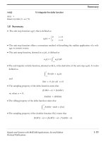
1.6 Summary 1−22
1.7 Exercises 1−23
1.8 Solutions to End−of−Chapter Exercises 1−24
MATLAB Computing
Pages 1−20, 1−21
Simulink Modeling
Page 1−18

2 The Laplace Transformation 2−1
2.1 Definition of the Laplace Transformation 2−1
2.2 Properties and Theorems of the Laplace Transform 2−2
2.2.1 Linearity Property 2−3
2.2.2 Time Shifting Property 2−3
2.2.3 Frequency Shifting Property 2−4
2.2.4 Scaling Property 2−4
2.2.5 Differentiation in Time Domain Property 2−4
2.2.6 Differentiation in Complex Frequency Domain Property 2
−6
2.2.7 Integration in Time Domain Property 2−6
2.2.8 Integration in Complex Frequency Domain Property 2
−8
2.2.9 Time Periodicity Property 2
−8
2.2.10 Initial Value Theorem 2
−9
2.2.11 Final Value Theorem 2−10
2.2.12 Convolution in Time Domain Property 2
−11
2.2.13 Convolution in Complex Frequency Domain Property 2
−12
2.3 The Laplace Transform of Common Functions of Time 2−14
2.3.1 The Laplace Transform of the Unit Step Function 2
−14
2.3.2 The Laplace Transform of the Ramp Function 2
−14
2.3.3 The Laplace Transform of 2
−15
u

0
t()
u
1
t()
t
n
u
0
t()

ii
Signals and Systems with MATLAB
®
Computing and Simulink
®
Modeling, Third Edition
Copyright © Orchard Publications
2.3.4 The Laplace Transform of the Delta Function 2−18
2.3.5 The Laplace Transform of the Delayed Delta Function 2−18
2.3.6 The Laplace Transform of 2−19
2.3.7 The Laplace Transform of 2−19
2.3.8 The Laplace Transform of 2−20
2.3.9 The Laplace Transform of 2−20
2.3.10 The Laplace Transform of 2−21
2.3.11 The Laplace Transform of 2−22
2.4 The Laplace Transform of Common Waveforms 2−23
2.4.1 The Laplace Transform of a Pulse 2−23
2.4.2 The Laplace Transform of a Linear Segment 2−23
2.4.3 The Laplace Transform of a Triangular Waveform 2−24

2.4.4 The Laplace Transform of a Rectangular Periodic Waveform 2−25
2.4.5 The Laplace Transform of a Half−Rectified Sine Waveform 2−26
2.5 Using MATLAB for Finding the Laplace Transforms of Time Functions 2−27
2.6 Summary 2−28
2.7 Exercises 2−31
The Laplace Transform of a Sawtooth Periodic Waveform 2−32
The Laplace Transform of a Full−Rectified Sine Waveform 2−32
2.8 Solutions to End−of−Chapter Exercises 2−33
3 The Inverse Laplace Transform 3−1
3.1 The Inverse Laplace Transform Integral 3−1
3.2 Partial Fraction Expansion 3−1
3.2.1 Distinct Poles 3−2
3.2.2 Complex Poles 3−5
3.2.3 Multiple (Repeated) Poles 3−8
3.3 Case where F(s) is Improper Rational Function 3
−13
3.4 Alternate Method of Partial Fraction Expansion 3−15
3.5 Summary 3
−19
3.6 Exercises 3
−21
3.7 Solutions to End−of−Chapter Exercises 3−22
MATLAB Computing
Pages 3
−3, 3−4, 3−5, 3−6, 3−8, 3−10, 3−12, 3−13, 3−14, 3−22
4 Circuit Analysis with Laplace Transforms 4−1
4.1 Circuit Transformation from Time to Complex Frequency 4
−1
4.1.1 Resistive Network Transformation 4−1
4.1.2 Inductive Network Transformation 4−1

4.1.3 Capacitive Network Transformation 4
−1
δ t()
δ ta–()
e
at–
u
0
t()
t
n
e
at–
u
0
t()
ωt u
0
tsin
ωcos t u
0
t
e
at–
ωt u
0
sin t()
e
at–
ωcos t u

0
t()
Signals and Systems with MATLAB
®
Computing and Simulink
®
Modeling, Third Edition iii
Copyright © Orchard Publications
4.2 Complex Impedance Z(s) 4−8
4.3 Complex Admittance Y(s) 4−11
4.4 Transfer Functions 4−13
4.5 Using the Simulink Transfer Fcn Block 4−17
4.6 Summary 4−20
4.7 Exercises 4−21
4.8 Solutions to End−of−Chapter Exercises 4−24
MATLAB Computing
Pages 4−6, 4−8, 4−12, 4−16, 4−17, 4−18, 4−26, 4−27, 4−28, 4−29, 4−34
Simulink Modeling
Page 4−17
5 State Variables and State Equations 5−1
5.1 Expressing Differential Equations in State Equation Form 5−1
5.2 Solution of Single State Equations 5−6
5.3 The State Transition Matrix 5−9
5.4 Computation of the State Transition Matrix 5−11
5.4.1 Distinct Eigenvalues 5−11
5.4.2 Multiple (Repeated) Eigenvalues 5−15
5.5 Eigenvectors 5−18
5.6 Circuit Analysis with State Variables 5−22
5.7 Relationship between State Equations and Laplace Transform 5−30
5.8 Summary 5−38

5.9 Exercises 5−41
5.10 Solutions to End−of−Chapter Exercises 5−43
MATLAB Computing
Pages 5
−14, 5−15, 5−18, 5−26, 5−36, 5−48, 5−51
Simulink Modeling
Pages 5−27, 5−37, 5−45
6 The Impulse Response and Convolution 6−1
6.1 The Impulse Response in Time Domain 6−1
6.2 Even and Odd Functions of Time 6
−4
6.3 Convolution 6−7
6.4 Graphical Evaluation of the Convolution Integral 6
−8
6.5 Circuit Analysis with the Convolution Integral 6
−18
6.6 Summary 6
−21
6.7 Exercises 6
−23

iv
Signals and Systems with MATLAB
®
Computing and Simulink
®
Modeling, Third Edition
Copyright © Orchard Publications
6.8 Solutions to End−of−Chapter Exercises 6−25
MATLAB Applications

Pages 6−12, 6−15, 6−30
7 Fourier Series 7−1
7.1 Wave Analysis 7−1
7.2 Evaluation of the Coefficients 7−2
7.3 Symmetry in Trigonometric Fourier Series 7−6
7.3.1 Symmetry in Square Waveform 7−8
7.3.2 Symmetry in Square Waveform with Ordinate Axis Shifted 7−8
7.3.3 Symmetry in Sawtooth Waveform 7−9
7.3.4 Symmetry in Triangular Waveform 7−9
7.3.5 Symmetry in Fundamental, Second, and Third Harmonics 7−10
7.4 Trigonometric Form of Fourier Series for Common Waveforms 7−10
7.4.1 Trigonometric Fourier Series for Square Waveform 7−11
7.4.2 Trigonometric Fourier Series for Sawtooth Waveform 7−14
7.4.3 Trigonometric Fourier Series for Triangular Waveform 7−16
7.4.4 Trigonometric Fourier Series for Half−Wave Rectifier Waveform 7−17
7.4.5 Trigonometric Fourier Series for Full−Wave Rectifier Waveform 7−20
7.5 Gibbs Phenomenon 7−24
7.6 Alternate Forms of the Trigonometric Fourier Series 7−24
7.7 Circuit Analysis with Trigonometric Fourier Series 7−28
7.8 The Exponential Form of the Fourier Series 7−31
7.9 Symmetry in Exponential Fourier Series 7−33
7.9.1 Even Functions 7−33
7.9.2 Odd Functions 7−34
7.9.3 Half-Wave Symmetry 7−34
7.9.4 No Symmetry 7−34
7.9.5 Relation of to 7
−34
7.10 Line Spectra 7−36
7.11 Computation of RMS Values from Fourier Series 7
−41

7.12 Computation of Average Power from Fourier Series 7
−44
7.13 Evaluation of Fourier Coefficients Using Excel® 7−46
7.14 Evaluation of Fourier Coefficients Using MATLAB® 7
−47
7.15 Summary 7
−50
7.16 Exercises 7−53
7.17 Solutions to End
−of−Chapter Exercises 7−55
MATLAB Computing
Pages 7−38, 7−47
C
n–
C
n
Signals and Systems with MATLAB
®
Computing and Simulink
®
Modeling, Third Edition v
Copyright © Orchard Publications
Simulink Modeling
Page 7−31
8 The Fourier Transform 8−1
8.1 Definition and Special Forms 8−1
8.2 Special Forms of the Fourier Transform 8−2
8.2.1 Real Time Functions 8−3
8.2.2 Imaginary Time Functions 8−6
8.3 Properties and Theorems of the Fourier Transform 8−9

8.3.1 Linearity 8−9
8.3.2 Symmetry 8−9
8.3.3 Time Scaling 8−10
8.3.4 Time Shifting 8−11
8.3.5 Frequency Shifting 8−11
8.3.6 Time Differentiation 8−12
8.3.7 Frequency Differentiation 8−13
8.3.8 Time Integration 8−13
8.3.9 Conjugate Time and Frequency Functions 8−13
8.3.10 Time Convolution 8−14
8.3.11 Frequency Convolution 8−15
8.3.12 Area Under 8−15
8.3.13 Area Under 8−15
8.3.14 Parseval’s Theorem 8−16
8.4 Fourier Transform Pairs of Common Functions 8−18
8.4.1 The Delta Function Pair 8−18
8.4.2 The Constant Function Pair 8−18
8.4.3 The Cosine Function Pair 8−19
8.4.4 The Sine Function Pair 8−20
8.4.5 The Signum Function Pair 8−20
8.4.6 The Unit Step Function Pair 8
−22
8.4.7 The Function Pair 8−24
8.4.8 The Function Pair 8−24
8.4.9 The Function Pair 8−25
8.5 Derivation of the Fourier Transform from the Laplace Transform 8−25
8.6 Fourier Transforms of Common Waveforms 8
−27
8.6.1 The Transform of 8−27
8.6.2 The Transform of 8

−28
8.6.3 The Transform of 8−29
ft()
F ω()
e
jω
0
t–
u
0
t()
ω
0
tcos()u
0
t()
ω
0
sin t()u
0
t()
ft()
A u
0
t T+()u
0
t T–()–[]=
ft()
A u
0

t() u
0
t 2T–()–[]=
ft()
A u
0
t T+()u+
0
t() u
0
t T–()– u
0
t 2T–()–[]=

vi
Signals and Systems with MATLAB
®
Computing and Simulink
®
Modeling, Third Edition
Copyright © Orchard Publications
8.6.4 The Transform of 8−30
8.6.5 The Transform of a Periodic Time Function with Period T 8−31
8.6.6 The Transform of the Periodic Time Function 8−32
8.7 Using MATLAB for Finding the Fourier Transform of Time Functions 8−33
8.8 The System Function and Applications to Circuit Analysis 8−34
8.9 Summary 8−42
8.10 Exercises 8−47
8.11 Solutions to End−of−Chapter Exercises 8−49
MATLAB Computing

Pages 8−33, 8−34, 8−50, 8−54, 8−55, 8−56, 8−59, 8−60
9 Discrete−Time Systems and the Z Transform 9−1
9.1 Definition and Special Forms of the Z Transform 9−1
9.2 Properties and Theorems of the Z Transform 9−3
9.2.1 Linearity 9−3
9.2.2 Shift of in the Discrete−Time Domain 9−3
9.2.3 Right Shift in the Discrete−Time Domain 9−4
9.2.4 Left Shift in the Discrete−Time Domain 9−5
9.2.5 Multiplication by in the Discrete−Time Domain 9−6
9.2.6 Multiplication by in the Discrete−Time Domain 9−6
9.2.7 Multiplication by and in the Discrete−Time Domain 9−6
9.2.8 Summation in the Discrete−Time Domain 9−7
9.2.9 Convolution in the Discrete
−Time Domain 9−8
9.2.10 Convolution in the Discrete
−Frequency Domain 9−9
9.2.11 Initial Value Theorem 9
−9
9.2.12 Final Value Theorem 9−10
9.3 The Z Transform of Common Discrete
−Time Functions 9−11
9.3.1 The Transform of the Geometric Sequence 9
−11
9.3.2 The Transform of the Discrete−Time Unit Step Function 9−14
9.3.3 The Transform of the Discrete
−Time Exponential Sequence 9−16
9.3.4 The Transform of the Discrete
−Time Cosine and Sine Functions 9−16
9.3.5 The Transform of the Discrete
−Time Unit Ramp Function 9−18

9.4 Computation of the Z Transform with Contour Integration 9−20
9.5 Transformation Between s
− and z−Domains 9−22
9.6 The Inverse Z Transform 9−25
ft() A ω
0
tu
0
t T+()u
0
t T–()–[]cos=
ft() A
δ tnT–()
n ∞–=
∞
∑
=
fn[]u
0
n[]
a
n
e
naT–
nn
2
Signals and Systems with MATLAB
®
Computing and Simulink
®

Modeling, Third Edition vii
Copyright © Orchard Publications
9.6.1 Partial Fraction Expansion 9−25
9.6.2 The Inversion Integral 9−32
9.6.3 Long Division of Polynomials 9−36
9.7 The Transfer Function of Discrete−Time Systems 9−38
9.8 State Equations for Discrete−Time Systems 9−45
9.9 Summary 9−48
9.10 Exercises 9−53
9.11 Solutions to End−of−Chapter Exercises 9−55
MATLAB Computing
Pages 9−35, 9−37, 9−38, 9−41, 9−42, 9−59, 9−61
Simulink Modeling
Page 9−44
Excel Plots
Pages 9−35, 9−44
10 The DFT and the FFT Algorithm 10−1
10.1 The Discrete Fourier Transform (DFT) 10−1
10.2 Even and Odd Properties of the DFT 10−9
10.3 Common Properties and Theorems of the DFT 10−10
10.3.1 Linearity 10−10
10.3.2 Time Shift 10−11
10.3.3 Frequency Shift 10−12
10.3.4 Time Convolution 10−12
10.3.5 Frequency Convolution 10−13
10.4 The Sampling Theorem 10−13
10.5 Number of Operations Required to Compute the DFT 10−16
10.6 The Fast Fourier Transform (FFT) 10
−17
10.7 Summary 10−28

10.8 Exercises 10
−31
10.9 Solutions to End
−of−Chapter Exercises 10−33
MATLAB Computing
Pages 10
−5, 10−7, 10−34
Excel Analysis ToolPak
Pages 10−6, 10−8
11 Analog and Digital Filters
11.1 Filter Types and Classifications 11
−1
11.2 Basic Analog Filters 11−2

viii
Signals and Systems with MATLAB
®
Computing and Simulink
®
Modeling, Third Edition
Copyright © Orchard Publications
11.2.1 RC Low−Pass Filter 11−2
11.2.2 RC High−Pass Filter 11−4
11.2.3 RLC Band−Pass Filter 11−7
11.2.4 RLC Band−Elimination Filter 11−8
11.3 Low−Pass Analog Filter Prototypes 11−10
11.3.1 Butterworth Analog Low−Pass Filter Design 11−14
11.3.2 Chebyshev Type I Analog Low−Pass Filter Design 11−25
11.3.3 Chebyshev Type II Analog Low−Pass Filter Design 11−38
11.3.4 Elliptic Analog Low−Pass Filter Design 11−39

11.4 High−Pass, Band−Pass, and Band−Elimination Filter Design 11−41
11.5 Digital Filters 11−51
11.6 Digital Filter Design with Simulink 11−70
11.6.1 The Direct Form I Realization of a Digital Filter 11−70
11.6.2 The Direct Form II Realization of a Digital Filter 11−71
11.6.3 The Series Form Realization of a Digital Filter 11−73
11.6.4 The Parallel Form Realization of a Digital Filter 11−75
11.6.5 The Digital Filter Design Block 11−78
11.7 Summary 11−87
11.8 Exercises 11−91
11.9 Solutions to End−of−Chapter Exercises 11−97
MATLAB Computing
Pages 11−3, 11−4, 11−6, 11−7, 11−9, 11−15, 11−19, 11−23, 11−24, 11−31,
11−35, 11−36, 11−37, 11−38, 11−40, 11−41, 11−42, 11−43, 11−45, 11−46,
11−48, 11−50, 11−55, 11−56, 11−57, 11−60, 11−62, 11−64, 11−67, 11−68,
and 11−97 through 11−106
Simulink Modeling
Pages 11−71, 11−74, 11−77, 11−78, 11−80, 11−82, 11−83, 11−84
A Introduction to MATLAB A−1
A.1 MATLAB® and Simulink® A−1
A.2 Command Window A−1
A.3 Roots of Polynomials A
−3
A.4 Polynomial Construction from Known Roots A
−4
A.5 Evaluation of a Polynomial at Specified Values A−6
A.6 Rational Polynomials A
−8
A.7 Using MATLAB to Make Plots A
−10

A.8 Subplots A
−18
A.9 Multiplication, Division, and Exponentiation A−18
A.10 Script and Function Files A−26
A.11 Display Formats A
−31
Signals and Systems with MATLAB
®
Computing and Simulink
®
Modeling, Third Edition ix
Copyright © Orchard Publications
MATLAB Computing
Pages A−3 through A−8, A−10, A−13, A−14, A−16, A−17,
A−21, A−22, A−24, A−27
B Introduction to Simulink B−1
B.1 Simulink and its Relation to MATLAB B−1
B.2 Simulink Demos B−20
MATLAB Computing
Page B−4
Simulink Modeling
Pages B−7, B−12, B−14, B−18
C A Review of Complex Numbers C−1
C.1 Definition of a Complex Number C−1
C.2 Addition and Subtraction of Complex Numbers C−2
C.3 Multiplication of Complex Numbers C−3
C.4 Division of Complex Numbers C−4
C.5 Exponential and Polar Forms of Complex Numbers C−4
MATLAB Computing
Pages C−6, C−7, C−8

Simulink Modeling
Page C−7
D Matrices and Determinants D−1
D.1 Matrix Definition D−1
D.2 Matrix Operations D−2
D.3 Special Forms of Matrices D
−6
D.4 Determinants D−10
D.5 Minors and Cofactors D
−12
D.6 Cramer’s Rule D
−17
D.7 Gaussian Elimination Method D
−19
D.8 The Adjoint of a Matrix D−21
D.9 Singular and Non
−Singular Matrices D−21
D.10 The Inverse of a Matrix D
−22
D.11 Solution of Simultaneous Equations with Matrices D−24
D.12 Exercises D
−31

x
Signals and Systems with MATLAB
®
Computing and Simulink
®
Modeling, Third Edition
Copyright © Orchard Publications

MATLAB Computing
Pages D−3, D−4, D−5, D−7, D−8, D−9, D−10,
D−12, D−19, D−23, D−27, D−29
Simulink Modeling
Page D−3
Excel Spreadsheet
Page D−28
References R−1
Index IN−1
Signals and Systems with MATLAB
®
Computing and Simulink
®
Modeling, Third Edition 1−1
Copyright © Orchard Publications
Chapter 1
Elementary Signals
his chapter begins with a discussion of elementary signals that may be applied to electric
networks. The unit step, unit ramp, and delta functions are then introduced. The sampling
and sifting properties of the delta function are defined and derived. Several examples for
expressing a variety of waveforms in terms of these elementary signals are provided. Throughout
this text, a left justified horizontal bar will denote the beginning of an example, and a right justi-
fied horizontal bar will denote the end of the example. These bars will not be shown whenever an
example begins at the top of a page or at the bottom of a page. Also, when one example follows
immediately after a previous example, the right justified bar will be omitted.
1.1 Signals Described in Math Form
Consider the network of Figure 1.1 where the switch is closed at time .
Figure 1.1. A switched network with open terminals
We wish to describe in a math form for the time interval . To do this, it is conve-
nient to divide the time interval into two parts, , and .

For the time interval
, the switch is open and therefore, the output voltage is zero.
In other words,
(1.1)
For the time interval
,
the switch is closed. Then, the input voltage appears at the
output, i.e.,
(1.2)
Combining (1.1) and (1.2) into a single relationship, we obtain
(1.3)
T
t0=
+
−
+
−
v
out
v
S
t0=
R
open terminals
v
out
∞ t+∞<<–
∞ t0<<– 0t∞<<
∞ t0<<– v
out

v
out
0 for ∞ t0 <<–=
0t∞<< v
S
v
out
v
S
for 0 t ∞ <<=
v
out
0 ∞– t0<<
v
S
0t∞<<
⎩
⎨
⎧
=






Chapter 1 Elementary Signals
1
−2 Signals and Systems with MATLAB
®

Computing and Simulink
®
Modeling, Third Edition
Copyright © Orchard Publications
We can express (1.3) by the waveform shown in Figure 1.2.
Figure 1.2. Waveform for as defined in relation (1.3)
The waveform of Figure 1.2 is an example of a discontinuous function. A function is said to be dis-
continuous if it exhibits points of discontinuity, that is, the function jumps from one value to
another without taking on any intermediate values.
1.2 The Unit Step Function
A well known discontinuous function is the unit step function
*
which is defined as
(1.4)
It is also represented by the waveform of Figure 1.3.
Figure 1.3. Waveform for
In the waveform of Figure 1.3, the unit step function changes abruptly from to at
. But if it changes at instead, it is denoted as . In this case, its waveform and
definition are as shown in Figure 1.4 and relation (1.5) respectively.
Figure 1.4. Waveform for
* In some books, the unit step function is denoted as , that is, without the subscript 0. In this text, however, we
will reserve the designation for any input when we will discuss state variables in Chapter 5.
0
v
out
v
S
t
v
out

u
0
t()
u
0
t()
ut()
ut()
u
0
t()
0t0<
1t0>
⎩
⎨
⎧
=
u
0
t()
0
1
t
u
0
t()
u
0
t() 01
t0= tt

0
= u
0
tt
0
–()
1
t
0
0
u
0
tt
0
–()
t
u
0
tt
0
–()
Signals and Systems with MATLAB
®
Computing and Simulink
®
Modeling, Third Edition 1−3
Copyright © Orchard Publications
The Unit Step Function
(1.5)
If the unit step function changes abruptly from to at , it is denoted as . In

this case, its waveform and definition are as shown in Figure 1.5 and relation (1.6) respectively.
Figure 1.5. Waveform for
(1.6)
Example 1.1
Consider the network of Figure 1.6, where the switch is closed at time .
Figure 1.6. Network for Example 1.1
Express the output voltage as a function of the unit step function, and sketch the appropriate
waveform.
Solution:
For this example, the output voltage for , and for . Therefore,
(1.7)
and the waveform is shown in Figure 1.7.
u
0
tt
0
–()
0tt
0
<
1tt
0
>
⎩
⎨
⎧
=
01t t
0
–= u

0
tt
0
+()
t
−t
0
0
1
u
0
tt
0
+()
u
0
tt
0
+()
u
0
tt
0
+()
0tt
0
–<
1tt
0
–>

⎩
⎨
⎧
=
tT=
+
−
+
−
v
out
v
S
tT=
R
open terminals
v
out
v
out
0= tT< v
out
v
S
= tT>
v
out
v
S
u

0
tT–()=
Chapter 1 Elementary Signals
1
−4 Signals and Systems with MATLAB
®
Computing and Simulink
®
Modeling, Third Edition
Copyright © Orchard Publications
Figure 1.7. Waveform for Example 1.1
Other forms of the unit step function are shown in Figure 1.8.
Figure 1.8. Other forms of the unit step function
Unit step functions can be used to represent other time−varying functions such as the rectangular
pulse shown in Figure 1.9.
Figure 1.9. A rectangular pulse expressed as the sum of two unit step functions
T
t
0
v
S
u
0
tT–()
v
out
0
t
t
t

t
Τ
−Τ
0
0
0
0
Τ
0
0
t
t
t
0
0
t
t
−Τ
−Τ
Τ
(a)
(b)
(c)
(d)
(e)
(f)
(g)
(h)
(i)
−A

−A
−A
−A
−A
−A
A
A
A
Au
0
t–()
A– u
0
t()
A– u
0
tT–()
A– u
0
tT+()
Au
0
t– T+()
Au
0
t– T–()
A– u
0
t–()
A– u

0
t– T+()
A– u
0
t– T–()
0
0
0
t
t
t
1
1
1
u
0
t()
u
0
t1–()–
a()
b()
c()
Signals and Systems with MATLAB
®
Computing and Simulink
®
Modeling, Third Edition 1−5
Copyright © Orchard Publications
The Unit Step Function

Thus, the pulse of Figure 1.9(a) is the sum of the unit step functions of Figures 1.9(b) and 1.9(c)
and it is represented as .
The unit step function offers a convenient method of describing the sudden application of a volt-
age or current source. For example, a constant voltage source of applied at , can be
denoted as . Likewise, a sinusoidal voltage source that is applied to
a circuit at , can be described as . Also, if the excitation in a
circuit is a rectangular, or triangular, or sawtooth, or any other recurring pulse, it can be repre-
sented as a sum (difference) of unit step functions.
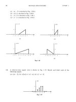
Example 1.2
Express the square waveform of Figure 1.10 as a sum of unit step functions. The vertical dotted
lines indicate the discontinuities at , and so on.
Figure 1.10. Square waveform for Example 1.2
Solution:
Line segment has height , starts at , and terminates at . Then, as in Example 1.1, this
segment is expressed as
(1.8)
Line segment has height , starts at and terminates at . This segment is
expressed as
(1.9)
Line segment has height , starts at and terminates at . This segment is expressed
as
(1.10)
Line segment has height , starts at , and terminates at . It is expressed as
(1.11)
u
0
t() u
0
t1–()–
24 V t 0=

24u
0
t() Vvt() V
m
ωt Vcos=
tt
0
= vt() V
m
ωtcos()u
0
tt
0
–() V=
T2T3T,,
{
|
}
~
t
vt()
3T
A
0
A–
T2T
{
At0= tT=
v
1

t() Au
0
t() u
0
tT–()–[]=
|
A– tT= t2T=
v
2
t() A– u
0
tT–()u
0
t2T–()–[]=
}
At2T= t3T=
v
3
t() Au
0
t2T–()u
0
t3T–()–[]=
~
A– t3T= t4T=
v
4
t() A– u
0
t3T–()u

0
t4T–()–[]=
Chapter 1 Elementary Signals
1
−6 Signals and Systems with MATLAB
®
Computing and Simulink
®
Modeling, Third Edition
Copyright © Orchard Publications
Thus, the square waveform of Figure 1.10 can be expressed as the summation of (1.8) through
(1.11), that is,
(1.12)
Combining like terms, we obtain
(1.13)
Example 1.3
Express the symmetric rectangular pulse of Figure 1.11 as a sum of unit step functions.
Figure 1.11. Symmetric rectangular pulse for Example 1.3
Solution:
This pulse has height , starts at , and terminates at . Therefore, with refer-
ence to Figures 1.5 and 1.8 (b), we obtain
(1.14)
Example 1.4
Express the symmetric triangular waveform of Figure 1.12 as a sum of unit step functions.
Figure 1.12. Symmetric triangular waveform for Example 1.4
Solution:
vt() v
1
t() v
2

t() v
3
t() v
4
t()+++=
Au
0
t() u
0
tT–()–[]A– u
0
tT–()u
0
t2T–()–[]=
+A u
0
t2T–()u
0
t3T–()–[]A– u
0
t3T–()u
0
t4T–()–[]
vt() Au
0
t() 2u
0
tT–()– 2u
0
t2T–()2u

0
t3T–()– …++[]=
t
A
T– 2⁄
T2⁄
0
it()
AtT2⁄–= tT2⁄=
it() Au
0
t
T
2
+
⎝⎠
⎛⎞
Au
0
t
T
2
–
⎝⎠
⎛⎞
– Au
0
t
T
2

+
⎝⎠
⎛⎞
u
0
t
T
2
–
⎝⎠
⎛⎞
–==
t
1
0
T2⁄–
vt()
T2⁄
Signals and Systems with MATLAB
®
Computing and Simulink
®
Modeling, Third Edition 1−7
Copyright © Orchard Publications
The Unit Step Function
We first derive the equations for the linear segments and shown in Figure 1.13.
Figure 1.13. Equations for the linear segments of Figure 1.12
For line segment ,
(1.15)
and for line segment ,

(1.16)
Combining (1.15) and (1.16), we obtain
(1.17)
Example 1.5
Express the waveform of Figure 1.14 as a sum of unit step functions.
Figure 1.14. Waveform for Example 1.5
Solution:
{|
t
1
0
T2⁄–
vt()
T2⁄
|
2
T
– t1+
2
T

t1+
{
{
v
1
t()
2
T

t1+
⎝⎠
⎛⎞
u
0
t
T
2
+
⎝⎠
⎛⎞
u
0
t()–=
|
v
2
t()
2
T
– t1+
⎝⎠
⎛⎞
u
0
t() u
0
t
T
2

–
⎝⎠
⎛⎞
–=
vt() v
1
t() v
2
t()+=
2
T

t1+
⎝⎠
⎛⎞
u
0
t
T
2
+
⎝⎠
⎛⎞
u
0
t()–
2
T
– t1+
⎝⎠

⎛⎞
u
0
t() u
0
t
T
2
–
⎝⎠
⎛⎞
–+=
1
2
3
12
3
0
t
vt()
Chapter 1 Elementary Signals
1
−8 Signals and Systems with MATLAB
®
Computing and Simulink
®
Modeling, Third Edition
Copyright © Orchard Publications
As in the previous example, we first find the equations of the linear segments linear segments
and shown in Figure 1.15.

Figure 1.15. Equations for the linear segments of Figure 1.14
Following the same procedure as in the previous examples, we obtain
Multiplying the values in parentheses by the values in the brackets, we obtain
and combining terms inside the brackets, we obtain
(1.18)
Two other functions of interest are the unit ramp function, and the unit impulse or delta function.
We will introduce them with the examples that follow.
Example 1.6
In the network of Figure 1.16 is a constant current source and the switch is closed at time
. Express the capacitor voltage as a function of the unit step.
{
|
1
2
3
12
3
0
{
|
2t 1+
vt()
t
t– 3+
vt() 2t 1+()u
0
t() u
0
t1–()–[]3u
0

t1–()u
0
t2–()–[]+=
+ t– 3+()u
0
t2–()u
0
t3–()–[]
vt() 2t 1+()u
0
t() 2t 1+()u
0
t1–()– 3u
0
t1–()+=
3u
0
t2–()– t– 3+()u
0
t2–() t– 3+()u
0
t3–()–+
vt() 2t 1+()u
0
t() 2t 1+()– 3+[]u
0
t1–()+=
+ 3– t– 3+()+[]u
0
t2–() t– 3+()u

0
t3–()–
vt() 2t 1+()u
0
t() 2t 1–()u
0
t1–()– t– u
0
t2–()t3–()u
0
t3–()+=
i
S
t0= v
C
t()
Signals and Systems with MATLAB
®
Computing and Simulink
®
Modeling, Third Edition 1−9
Copyright © Orchard Publications
The Unit Step Function
Figure 1.16. Network for Example 1.6
Solution:
The current through the capacitor is , and the capacitor voltage is
*
(1.19)
where is a dummy variable.
Since the switch closes at , we can express the current as

(1.20)
and assuming that for , we can write (1.19) as
(1.21)
or
(1.22)
Therefore, we see that when a capacitor is charged with a constant current, the voltage across it is
a linear function and forms a ramp with slope as shown in Figure 1.17.
Figure 1.17. Voltage across a capacitor when charged with a constant current source
* Since the initial condition for the capacitor voltage was not specified, we express this integral with at the lower limit of
integration so that any non-zero value prior to would be included in the integration.
v
C
t()
t0=
i
S
R
C
−
+
i
C
t() i
S
cons ttan== v
C
t()
v
C
t()

1
C

i
C
τ()τd
∞–
t
∫
=
∞–
t0<
τ
t0=
i
C
t()
i
C
t() i
S
u
0
t()=
v
C
t() 0= t0<
v
C
t()

1
C

i
S
u
0
τ()τd
∞–
t
∫
i
S
C

u
0
τ()τd
∞–
0
∫
0
i
S
C

u
0
τ()τd
0

t
∫
+==
⎧
⎪
⎪
⎨
⎪
⎪
⎩
v
C
t()
i
S
C

tu
0
t()=
i
S
C⁄
v
C
t()
0
slope i
S
C⁄=

t