computational chemistry using the pc
Bạn đang xem bản rút gọn của tài liệu. Xem và tải ngay bản đầy đủ của tài liệu tại đây (2.02 MB, 361 trang )
Computational
Chemistry
Using the PC
Third Edition
Computational
Chemistry
Using the PC
Third Edition
Donald W. Rogers
A John Wiley & Sons, Inc., Publication
Copyright # 2003 by John Wiley & Sons, Inc. All rights reserved.
Published by John Wiley & Sons, Inc., Hoboken, New Jersey.
Published simultaneously in Canada.
No part of this publication may be reproduced, stored in a retrieval system, or transmitted in any
form or by any means, electronic, mechanical, photocopying, recording, scanning, or otherwise,
except as permitted under Section 107 or 108 of the 1976 United States Copyright Act, without
either the prior written permission of the Publisher, or authorization through payment of the
appropriate per-copy fee to the Copyright Clearance Center, Inc., 222 Rosewood Drive, Danvers,
MA 01923, 978-750-8400, fax 978-750-4470, or on the web at www.copyright.com. Requests to
the Publisher for permission should be addressed to the Permissions Department, John Wiley &
Sons, Inc., 111 River Street, Hoboken, NJ 07030, (201) 748-6011, fax (201) 748-6008,
e-mail:
Limit of Liability/Disclaimer of Warranty: While the publisher and author have used their best
efforts in preparing this book, they make no representations or warranties with respect to the
accuracy or completeness of the contents of this book and specifically disclaim any implied
warranties of merchantability or fitness for a particular purpose. No warranty may be created or
extended by sales representatives or written sales materials. The advice and strategies contained
herein may not be suitable for your situation. You should consult with a professional where
appropriate. Neither the publisher nor author shall be liable for any loss of profit or any other
commercial damages, including but not limited to special, incidental, consequential, or other
damages.
For general information on our other products and services please contact our Customer Care
Department within the U.S. at 877-762-2974, outside the U.S. at 317-572-3993 or fax 317-572-4002.
Wiley also publishes its books in a variety of electronic formats. Some content that appears in print,
however, may not be available in electronic format.
Library of Congress Cataloging-in-Publication Data:
Rogers, Donald, 1932–
Computational chemistry using the PC / Donald W. Rogers. – 3rd ed.
p. cm.
Includes Index.
ISBN 0-471-42800-0 (pbk.)
1. Chemistry–Data processing. 2. Chemistry–Mathematics. I. Title.
QD39.3.E46R64 1994
541.2
0
2
0
02855365—dc21 2003011758
Printed in the United States of America.
10987654321
Live joyfully with the wife whom thou lovest all the
days of the life of thy vanity, which He hath given
thee under the sun, all the days of thy vanity: for that
is thy portion in this life, and in thy labor which thou
takest under the sun.
Ecclesiastes 9:9
THIS BOOK IS DEDICATED TO KAY
Contents
Preface to the Third Edition xv
Preface to the Second Edition xvii
Preface to the First Edition xix
Chapter 1. Iterative Methods 1
Iterative Methods 1
An Iterative Algorithm 2
Blackbody Radiation 2
Radiation Density 3
Wien’s Law 4
The Planck Radiation Law 4
COMPUTER PROJECT 1-1 j Wien’s Law 5
COMPUTER PROJECT 1-2 j Roots of the Secular Determinant 6
The Newton–Raphson Method 7
Problems 9
Numerical Integration 9
Simpson’s Rule 10
vii
Efficiency and Machine Considerations 13
Elements of Single-Variable Statistics 14
The Gaussian Distribution 15
COMPUTER PROJECT 1-3 j Medical Statistics 17
Molecular Speeds 19
COMPUTER PROJECT 1-4 j Maxwell–Boltzmann
Distribution Laws 20
COMPUTER PROJECT 1-5 j Elementary Quantum Mechanics 23
COMPUTER PROJECT 1-6 j Numerical Integration of Experimental
Data Sets 24
Problems 29
Chapter 2. Applications of Matrix Algebra 31
Matrix Addition 31
Matrix Multiplication 33
Division of Matrices 34
Powers and Roots of Matrices 35
Matrix Polynomials 36
The Least Equation 37
Importance of Rank 38
Importance of the Least Equation 38
Special Matrices 39
The Transformation Matrix 41
Complex Matrices 42
What’s Going On Here? 42
Problems 44
Linear Nonhomogeneous Simultaneous Equations 45
Algorithms 47
Matrix Inversion and Diagonalization 51
COMPUTER PROJECT 2-1 j Simultaneous Spectrophotometric
Analysis 52
COMPUTER PROJECT 2-2 j Gauss–Seidel Iteration: Mass
Spectroscopy 54
COMPUTER PROJECT 2-3 j Bond Enthalpies of Hydrocarbons 56
Problems 57
Chapter 3. Curve Fitting 59
Information Loss 60
The Method of Least Squares 60
viii CONTENTS
Least Squares Minimization 61
Linear Functions Passing Through the Origin 62
Linear Functions Not Passing Through the Origin 63
Quadratic Functions 65
Polynomials of Higher Degree 68
Statistical Criteria for Curve Fitting 69
Reliability of Fitted Parameters 70
COMPUTER PROJECT 3-1 j Linear Curve Fitting: KF Solvation 73
COMPUTER PROJECT 3-2 j The Boltzmann Constant 74
COMPUTER PROJECT 3-3 j The Ionization Energy of Hydrogen 76
Reliability of Fitted Polynomial Parameters 76
COMPUTER PROJECT 3-4 j The Partial Molal Volume of ZnCl
2
77
Problems 79
Multivariate Least Squares Analysis 80
Error Analysis 86
COMPUTER PROJECT 3-5 j Calibration Surfaces Not Passing
Through the Origin 88
COMPUTER PROJECT 3-6 j Bond Energies of Hydrocarbons 89
COMPUTER PROJECT 3-7 j Expanding the Basis Set 90
Problems 90
Chapter 4. Molecular Mechanics: Basic Theory 93
The Harmonic Oscillator 93
The Two-Mass Problem 95
Polyatomic Molecules 97
Molecular Mechanics 98
Ethylene: A Trial Run 100
The Geo File 102
The Output File 103
TINKER 108
COMPUTER PROJECT 4-1 j The Geometry of Small Molecules 110
The GUI Interface 112
Parameterization 113
The Energy Equation 114
Sums in the Energy Equation: Modes of Motion 115
COMPUTER PROJECT 4-2 j The MM3 Parameter Set 117
CONTENTS ix
COMPUTER PROJECT 4-3 j The Butane Conformational Mix 125
Cross Terms 128
Problems 129
Chapter 5. Molecular Mechanics II: Applications 131
Coupling 131
Normal Coordinates 136
Normal Modes of Motion 136
An Introduction to Matrix Formalism for Two Masses 138
The Hessian Matrix 140
Why So Much Fuss About Coupling? 143
The Enthalpy of Formation 144
Enthalpy of Reaction 147
COMPUTER PROJECT 5-1 j The Enthalpy of Isomerization of
cis- and trans-2-Butene 148
Enthalpy of Reaction at Temperatures 6¼ 298 K 150
Population Energy Increments 151
Torsional Modes of Motion 153
COMPUTER PROJECT 5-2 j The Heat of Hydrogenation
of Ethylene 154
Pi Electron Calculations 155
COMPUTER PROJECT 5-3 j The Resonance Energy of Benzene 157
Strain Energy 158
False Minima 158
Dihedral Driver 160
Full Statistical Method 161
Entropy and Heat Capacity 162
Free Energy and Equilibrium 163
COMPUTER PROJECT 5-4 j More Complicated Systems 164
Problems 166
Chapter 6. Huckel Molecular Orbital Theory I: Eigenvalues 169
Exact Solutions of the Schroedinger Equation 170
Approximate Solutions 172
The Huckel Method 176
The Expectation Value of the Energy: The Variational Method 178
COMPUTER PROJECT 6-1 j Another Variational Treatment of the
Hydrogen Atom 181
x CONTENTS
Huckel Theory and the LCAO Approximation 183
Homogeneous Simultaneous Equations 185
The Secular Matrix 186
Finding Eigenvalues by Diagonalization 187
Rotation Matrices 188
Generalization 189
The Jacobi Method 191
Programs QMOBAS and TMOBAS 194
COMPUTER PROJECT 6-2 j Energy Levels (Eigenvalues) 195
COMPUTER PROJECT 6-3 j Huckel MO Calculations of
Spectroscopic Transitions 197
Problems 198
Chapter 7. Huckel Molecular Orbital Theory II: Eigenvectors 201
Recapitulation and Generalization 201
The Matrix as Operator 207
The Huckel Coefficient Matrix 207
Chemical Application: Charge Density 211
Chemical Application: Dipole Moments 213
Chemical Application: Bond Orders 214
Chemical Application: Delocalization Energy 215
Chemical Application: The Free Valency Index 217
Chemical Application: Resonance (Stabilization) Energies 217
LIBRARY PROJECT 7-1 j The History of Resonance and
Aromaticity 219
Extended Huckel Theory—Wheland’s Method 219
Extended Huckel Theory—Hoffman’s EHT Method 221
The Programs 223
COMPUTER PROJECT 7-1 j Larger Molecules: Calculations
using SHMO 225
COMPUTER PROJECT 7-2 j Dipole Moments 226
COMPUTER PROJECT 7-3 j Conservation of Orbital Symmetry 227
COMPUTER PROJECT 7-4 j Pyridine 228
Problems 229
Chapter 8. Self-Consistent Fields 231
Beyond Huckel Theory 231
Elements of the Secular Matrix 232
CONTENTS xi
The Helium Atom 235
A Self-Consistent Field Variational Calculation of
IP for the Helium Atom 236
COMPUTER PROJECT 8-1 j The SCF Energies of First Row
Atoms and Ions 240
COMPUTER PROJECT 8-2 j A High-Level ab initio Calculation of SCF
First IPs of the First Row Atoms 241
The STO-xG Basis Set 242
The Hydrogen Atom: An STO-1G ‘‘Basis Set’’ 243
Semiempirical Methods 248
PPP Self-Consistent Field Calculations 248
The PPP-SCF Method 249
Ethylene 252
Spinorbitals, Slater Determinants, and Configuration Interaction 255
The Programs 256
COMPUTER PROJECT 8-3 j SCF Calculations of Ultraviolet
Spectral Peaks 256
COMPUTER PROJECT 8-4 j SCF Dipole Moments 258
Problems 259
Chapter 9. Semiempirical Calculations on Larger Molecules 263
The Hartree Equation 263
Exchange Symmetry 266
Electron Spin 267
Slater Determinants 269
The Hartree–Fock Equation 273
The Fock Equation 276
The Roothaan–Hall Equations 278
The Semiempirical Model and Its Approximations:
MNDO, AM1, and PM3 279
The Programs 283
COMPUTER PROJECT 9-1 j Semiempirical Calculations on Small
Molecules: HF to HI 284
COMPUTER PROJECT 9-2 j Vibration of the Nitrogen Molecule 284
Normal Coordinates 285
Dipole Moments 289
COMPUTER PROJECT 9-3 j Dipole Moments (Again) 289
Energies of Larger Molecules 289
xii CONTENTS
COMPUTER PROJECT 9-4 j Large Molecules: Carcinogenesis 291
Problems 293
Chapter 10.
Ab Initio
Molecular Orbital Calculations 299
The GAUSSIAN Implementation 299
How Do We Determine Molecular Energies? 301
Why Is the Calculated Energy Wrong? 306
Can the Basis Set Be Further Improved? 306
Hydrogen 308
Gaussian Basis Sets 309
COMPUTER PROJECT 10-1 j Gaussian Basis Sets: The HF Limit 311
Electron Correlation 312
G2 and G3 313
Energies of Atomization and Ionization 315
COMPUTER PROJECT 10-2 j Larger Molecules: G2, G2(MP2), G3,
and G3(MP2) 316
The GAMESS Implementation 317
COMPUTER PROJECT 10-3 j The Bonding Energy Curve of H
2
:
GAMESS 318
The Thermodynamic Functions 319
Koopmans’s Theorem and Photoelectron Spectra 323
Larger Molecules I: Isodesmic Reactions 324
COMPUTER PROJECT 10-4 j Dewar Benzene 326
Larger Molecules II: Density Functional Theory 327
COMPUTER PROJECT 10-5 j Cubane 330
Problems 330
Bibliography 333
Appendix A. Software Sources 339
Index 343
CONTENTS xiii
Preface to the Third Edition
It is a truism (cliche?) that microcomputers have become more powerful on an
almost exponential curve since their advent more than 30 years ago. Molecular
orbital calculations that I ran on a supercomputer a decade ago now run on a fast
desktop microcomputer available at a modest price in any popular electronics store
or by mail order catalog. With this has come a comparable increase in software
sophistication.
There is a splendid democratization implied by mass-market computers. One
does not have to work at one of the world’s select universities or research institutes
to do world class research. Your research equipment now consists of an off-the-
shelf microcomputer and your imagination.
At the first edition of this book, in 1990, I made the extravigant claim that ‘‘a
quite respectable academic program in chemical microcomputing can be started for
about $1000 per student’’. The degree of difficulty of the problems we solve has
increased immeasurably since then but the price of starting a good teaching lab is
probably about half of what it was. To equip a workstation for two students, one
needs a microcomputer connected to the internet, a BASIC interpreter and a
beginner’s bundle of freeware which should include the utility programs suggested
with this book, a Huckel Molecular Orbital program, TINKER, MOPAC, and
GAMESS.
There are 42 Computer Projects included in this text. Several of the Computer
Projects connect with the research literature and lead to extensions suitable for
undergraduate or MS thesis projects. All of the computer projects in this book have
been successfully run by the author. Unfortunately, we still live in an era of system
incompatibility. The instructor using these projects in a teaching laboratory is urged
xv
to run them first to sort out any system specific difficulties. In this, the projects here
are no different from any undergraduate experiment; it is a foolish instructor indeed
who tries to teach from untested material.
The author wishes to acknowledge the unfailing help and constructive criticism
of Frank Mc Lafferty, the computer tips of Nikita Matsunaga and Xeru Li. Some of
the research which gave rise to Computer Projects in the latter half of the book were
carried out under a grant of computer time from the National Science Foundation
through the National Center for Supercomputing Applications both of which are
gratefully acknowledged.
Donald W. Rogers
Greenwich Village, NY
July 2003
xvi PREFACE TO THE THIRD EDITION
Preface to the Second Edition
A second edition always needs an excuse, particularly if it follows hard upon the
first. I take the obvious one: a lot has happened in microcomputational chemistry in
the last five years. Faster machines and better software have brought more than
convenience; there are projects in this book that we simply could not do at the time
of the first edition.
Along with the obligatory correction of errors in the first edition, this one has
five new computer projects (two in high-level ab initio calculations), and 49 new
problems, mostly advanced. Large parts of Chapters 9 and 10 have been rewritten,
more detailed instructions are given in many of the computer projects, and several
new illustrations have been added, or old ones have been redrawn for clarity. The
BASIC programs on the diskette included here have been translated into ASCII
code to improve portability, and each is written out at the end of the chapter in
which it is introduced. Several illustrative input and output files for Huckel, self-
consistent field, molecular mechanics, ab initio, and semiempirical procedures are
also on the disk, along with an answer section for problems and computer projects.
One thing has not changed. By shopping among the software sources at the end
of this book, and clipping popular computer magazine advertisements, the prudent
instructor can still equip his or her lab at a starting investment of about $2000 per
workstation of two students each.
xvii
Preface to the First Edition
This book is an introduction to computational chemistry, molecular mechanics, and
molecular orbital calculations, using a personal microcomputer. No special com-
putational skills are assumed of the reader aside from the ability to read and write a
simple program in BASIC. No mathematical training beyond calculus is assumed.
A few elements of matrix algebra are introduced in Chapter 3 and used throughout.
The treatment is at the upperclass undergraduate or beginning graduate level.
Considerable introductory material and material on computational methods are
given so as to make the book suitable for self-study by professionals outside
the classroom. An effort has been made to avoid logical gaps so that the
presentation can be understood without the aid of an instructor. Forty-six self-
contained computer projects are included.
The book divides itself quite naturally into two parts: The first six chapters are
on general scientific computing applications and the last seven chapters are devoted
to molecular orbital calculations, molecular mechanics, and molecular graphics.
The reader who wishes only a tool box of computational methods will find it in the
first part. Those skilled in numerical methods might read only the second. The book
is intended, however, as an entity, with many connections between the two parts,
showing how chapters on molecular orbital theory depend on computational
techniques developed earlier.
Use of special or expensive microcomputers has been avoided. All programs
presented have been run on a 8086-based machine with 640 K memory and a math
coprocessor. A quite respectable academic program in chemical microcomputing
can be started for about $1000 per student. The individual or school with more
expensive hardware will find that the programs described here run faster and that
xix
more visually pleasing graphics can be produced, but that the results and principles
involved are the same. Gains in computing speed and convenience will be made as
the technology advances. Even now, run times on an 80386-based machine
approach those of a heavily used, time-shared mainframe.
Sources for all program packages used in the book are given in an appendix. All
of the early programs (Chapters 1 through 7) were written by the author and are
available on a single diskette included with the book. Programs HMO and SCF
were adapted and modified by the author from programs in FORTRAN II by
Greenwood (Computational Methods for Quantum Organic Chemistry, Wiley
Interscience, New York, 1972). The more elaborate programs in Chapters 10
through 13 are available at moderate price from Quantum Chemistry Program
Exchange, Serena Software, Cambridge Analytical Laboratories and other software
sources [see Appendix].
I wish to thank Dr. A. Greenberg of Rutgers University, Dr. S. Topiol of Burlex
Industries, and Dr. A. Zavitsas of Long Island University for reading the entire
manuscript and offering many helpful comments and criticisms. I wish to acknowl-
edge Long Island University for support of this work through a grant of released
time and the National Science Foundation for microcomputers bought under grant
#CSI 870827.
Several chapters in this book are based on articles that appeared in American
Laboratory from 1981 to 1988. I wish to acknowledge my coauthors of these
papers, F. J. McLafferty, W. Gratzer, and B. P. Angelis. I wish to thank the editors of
American Laboratory, especially Brian Howard, for permission to quote extensively
from those articles.
xx PREFACE TO THE FIRST EDITION
CHAPTER
1
Iterative Methods
Some things are simple but hard to do.
—A. Einstein
Most of the problems in this book are simple. Many of the methods used have been
known for decades or for centuries. At the machine level, individual steps in the
procedures are at the grade school level of sophistication, like adding two numbers
or comparing two numbers to see which is larger. What makes them hard is that
there are very many steps, perhaps many millions. The computer, even the once
‘‘lowly’’ microcomputer, provides an entry into a new scientific world because of
its incredible speed. We are now in the enviable position of being able to arrive at
practical solutions to problems that we could once only imagine.
Iterative Methods
One of the most important methods of modern computation is solution by iteration.
The method has been known for a very long time but has come into widespread use
only with the modern computer. Normally, one uses iterative methods when
ordinary analytical mathematical methods fail or are too time-consuming to be
Computational Chemistry Using the PC, Third Edition, by Donald W. Rogers
ISBN 0-471-42800-0 Copyright # 2003 John Wiley & Sons, Inc.
1
practical. Even relatively simple mathematical procedures may be time-consuming
because of extensive algebraic manipulation.
A common iterative procedure is to solve the problem of interest by repeated
calculations that do not initially give the correct answer but get closer to it as the
calculation is repeated, perhaps many times. The approximate solution is said to
converge on the correct solution. Although no human would be willing to repeat an
iterative calculation thousands of times to converge on the right answer, the
computer does, and, because of its speed, it often arrives at the answer in a
reasonable amount of time.
An Iterative Algorithm
The first illustrative problem comes from quantum mechanics. An equation in
radiation density can be set up but not solved by conventional means. We shall
guess a solution, substitute it into the equation, and apply a test to see whether
the guess was right. Of course it isn’t on the first try, but a second guess can be
made and tested to see whether it is closer to the solution than the first. An iterative
routine can be set up to carry out very many guesses in a methodical way
until the test indicates that the solution has been approximated within some narrow
limit.
Several questions present themselves immediately: How good does the initial
guess have to be? How do we know that the procedure leads to better guesses, not
worse? How many steps (how long) will the procedure take? How do we know
when to stop? These questions and others like them will play an important role in
this book. You will not be surprised to learn that answers to questions like these
vary from one problem to another and cannot be set down once and for all. Let us
start with a famous problem in quantum mechanics: blackbody radiation.
Blackbody Radiation
We can sample the energy density of radiation rðn; TÞ within a chamber at a fixed
temperature T (essentially an oven or furnace) by opening a tiny transparent
window in the chamber wall so as to let a little radiation out. The amount of
radiation sampled must be very small so as not to disturb the equilibrium condition
inside the chamber. When this is done at many different frequencies n, the
blackbody spectrum is obtained. When the temperature is changed, the area under
the spectral curve is greater or smaller and the curve is displaced on the frequency
axis but its shape remains essentially the same. The chamber is called a blackbody
because, from the point of view of an observer within the chamber, radiation lost
through the aperture to the universe is perfectly absorbed; the probability of a
photon finding its way from the universe back through the aperture into the chamber
is zero.
2 COMPUTATIONAL CHEMISTRY USING THE PC
Radiation Density
If we think in terms of the particulate nature of light (wave-particle duality), the
number of particles of light or other electromagnetic radiation (photons) in a unit of
frequency space constitutes a number density. The blackbody radiation curve in
Fig. 1-1, a plot of radiation energy density r on the vertical axis as a function of
frequency n on the horizontal axis, is essentially a plot of the number densities of
light particles in small intervals of frequency space.
We are using the term space as defined by one or more coordinates that are not
necessarily the x, y, z Cartesian coordinates of space as it is ordinarily defined. We
shall refer to 1-space, 2-space, etc. where the number of dimensions of the space is
the number of coordinates, possibly an n-space for a many dimensional space.
The r and n axes are the coordinates of the density–frequency space, which is a
2-space.
Radiation energy density is a function of both frequency and temperature r(n,T)
so that the single curve in Fig. 1-1 implies one and only one temperature. Because
frequency n times wavelength l is the velocity of light c ¼ nl ¼ 2:998 10
8
ms
1
(a constant), an equivalent functional relationship exists between energy density
and wavelength. The energy density function can be graphed in a different but
equivalent form r(l,T). The intensity I of electromagnetic radiation within any
narrow frequency (or wavelength) interval is directly proportional to the number
density of photons. It is also directly proportional to the power output of a light
sensor or photomultiplier; hence both I and r are measurable quantities. Whenever
one plots some function of radiation intensity I vs. n or l, the resulting curve is
called a spectrum.
Frequency
Energy Density
, J
m
–3
Figure 1-1 The Blackbody Radiation Spectrum. The short curve on the left is a Rayleigh
function of frequency.
ITERATIVE METHODS 3
Wien’s Law
In the late nineteenth century, Wien analyzed experimental data on blackbody
radiation and found that the maximum of the blackbody radiation spectrum l
max
shifts with the temperature according to the equation
l
max
T ¼ 2:90 10
3
mK ð1-1Þ
where l is in meters and T is the temperature in kelvins.
The Planck Radiation Law
As Lord Rayleigh pointed out, the classical expression for radiation
rðn; TÞdn ¼ 8pk
B
T=c
3
n
2
dn ð1-2Þ
where k
B
is Boltzmann’s constant and c is the speed of light, must fail to express the
blackbody radiation spectrum because r ¼ const: n
2
is a segment of a parabola
open upward (the short curve to the left in Fig. 1-1) and does not have a relative
maximum as required by the experimental data. In late 1900, Max Planck presented
the equation
rðn; TÞdn ¼ 8phn=c
3
n
2
dn
e
hn=k
B
T
1
ð1-3Þ
where the units of rðn; TÞ are joules per cubic meter, as appropriate to an energy in
joules per unit volume and h ¼ 6: 626 10
34
J s (joule seconds) is a new constant,
now called Planck’s constant. This equation expressed in terms of wavelength l is
rðl; TÞdl ¼ 8phc=l
5
dl
e
hc=lk
B
T
1
ð1-4Þ
By setting dr=dl ¼ 0, one can differentiate Eq. (1-4) and show that the equation
e
x
þ
x
5
¼ 1 ð1-5Þ
holds at the maximum of Fig. 1-1 where
x ¼
hc
lk
B
T
ð1-6Þ
Exercise 1-1
Given that c ¼ nl, show that Eqs. (1-3) and 1-4) are equivalent.
Exercise 1-2
Obtain Eq. (1-5) from Eq. (1-4).
4 COMPUTATIONAL CHEMISTRY USING THE PC
COMPUTER PROJECT 1-1
Wien’s Law
The first computer project is devoted to solving Eq. (1-5) for x iteratively. When
x has been determined, the remaining constants can be substituted into
lT ¼
hc
k
B
x
ð1-7Þ
where h is Planck’s constant, c is the velocity of light in a vacuum, 2:998
10
8
ms
1
, and k
B
¼ 1:381 10
23
JK
1
is the Boltzmann constant. The result is a
test of agreement between Planck’s theoretical quantum law and Wien’s displace-
ment law [Eq. 1-1], which comes from experimental data.
Procedure. One approach to the problem is to select a value for x that is obviously
too small and to increment it iteratively until the equation is satisfied. This is the
method of program WIEN, where the initial value of x is taken as 1 (clearly,
e
1
þ
1
5
< 1 as you can show with a hand calculator).
Program
PRINT ‘‘Program QWIEN’’
x=1
10 x = x þ.1
a = EXP(-x) þ(x / 5)
IF (a 1) < 0 THEN 10
PRINT a, x
END
In Program QWIEN (written in QBASIC, Appendix A), x is initialized at 1 and
incremented by 0.1 in line 3, which is given the statement number 10 for future
reference. Be careful to differentiate between a statement number like 10 x ¼ x þ.1
and the product 10 times x which is 10*x. A number a is calculated for x ¼ 1:1 that
is obviously too small so (a 1) is less than 0 and the IF statement in line 5 sends
control back to the statement numbered 10, which increments x by 0.1 again. This
continues until (a 1) 0, whereupon control exits from the loop and prints the
result for a and x.
There are, of course, many variations that can be written in place of Program
QWIEN. You are urged to try as many as you can. Some suggestions are as follows:
a. Vary the size of the increment in x in program statement 10. Tabulate the
increment size, the computed result for x, and the calculated Wien constant.
Comment on the relationship among the quantities tabulated.
b. Change Program QWIEN so that the second term on the right of the line below
statement 10 is x instead of x=5. Solve for this new equation. Change the line
below statement 10 so that the second term on the left is x=2. Repeat with x=3,
x=4, etc. Tabulate the values of x and the values of the denominator. Is x a
sensitive function of the denominator in the second term of Program WIEN?
ITERATIVE METHODS 5
c. Devise and discuss a scheme for more efficient convergence. For example,
some scheme that uses large increments for x when x is far away from
convergence and small values for the increment in x when x is near its true
value would be more efficient than the preceding schemes. How, in more detail,
could this be done? Try coding and running your scheme.
d. Another coding scheme can be used in True BASIC (Appendix A)
Program
PRINT ‘‘Program TWIEN’’
let X ¼1
do
let X ¼X þ.1
let A ¼exp(-X) þX/5
loop until (A 1) > 0
PRINT A, X
END
The program contains a ‘‘do loop’’ that iterates the statements within the loop until
the condition (A 1) < 0 is true. Try moving the ‘‘do’’ statement around in the
program to see what changes in the output. Explain. If you encounter an ‘‘infinite
loop,’’ True BASIC has a STOP statement to get you out.
It is good practice to translate programs in one BASIC (QBASIC or True
BASIC) to programs in the other if you have both interpreters. Note that the
statement X ¼X þ.1 in both programs makes no sense algebraically, but in BASIC
it means, ‘‘take the number in memory register X, add 0.1 to it and store the result
back in register X.’’ If you are not familiar with coding in BASIC, an hour or so
with an instruction manual should suffice for the simple programs used in the first
half of this book. By all means, look at the programs on the Wiley website.
COMPUTER PROJECT 1-2
Roots of the Secular Determinant
Later in this book, we shall need to find the roots of the secular matrix
210 42x 42 9x
42 9x 12 2x
ð1-8Þ
One way of obtaining the roots is to expand the determinantal equation
210 42x 42 9x
42 9x 12 2x
¼ 0 ð1-9Þ
To do this, multiply the binomials at the top left and bottom right (the principal
diagonal) and then, from this product, subtract the product of the remaining two
elements, the off-diagonal elements ð42 9xÞ. The difference is set equal to zero:
ð210 42xÞð12 2xÞð42 9xÞ
2
¼ 0 ð1-10Þ
6 COMPUTATIONAL CHEMISTRY USING THE PC
This equation is a quadratic and has two roots. For quantum mechanical reasons, we
are interested only in the lower root. By inspection, x ¼ 0 leads to a large number
on the left of Eq. (1-10). Letting x ¼ 1 leads to a smaller number on the left of
Eq. (1-10), but it is still greater than zero. Evidently, increasing x approaches
a solution of Eq. (1-10), that is, a value of x for which both sides are equal. By
systematically increasing x beyond 1, we will approach one of the roots of the
secular matrix. Negative values of x cause the left side of Eq. (1-10) to increase
without limit; hence the root we are approaching must be the lower root.
Program
PRINT ‘‘Program QROOT’’
x ¼0
20 x ¼ x þ 1
a ¼(210 - 42 * x) * (12 - 2 * x) - (42 - 9 * x)
^
2
IF a > 0 GOTO 20
PRINT x: END
Program QROOT increments x by 1 on each iteration. It prints out 5 when the
polynomial on the right of line 4 is greater than 0. We have gone past the root
because x is too large. The program did not exit from the loop on x ¼ 4, but it did
on x ¼ 5, so x is between 4 and 5. By letting x ¼ 4 in the second line and changing
the third line to increment x by 0.1, we get 5 again so x is between 4.9 and 5.0.
Letting x ¼ 4:9 with an increment of 0.01 yields 4.94 and so on, until the increment
0.00001 yields the lower root x ¼ 4:93488.
Although we will not need it for our later quantum mechanical calculation, we
may be curious to evaluate the second root and we shall certainly want to check to
be sure that the root we have found is the smaller of the two. Write a program to
evaluate the left side of Eq. (1-10) at integral values between 1 and 100 to make an
approximate location of the second root. Write a second program to locate the
second root of matrix Eq. (1-10) to a precision of six digits. Combine the programs
to obtain both roots from one program run.
The Newton Raphson Method
The root-finding method used up to this point was chosen to illustrate iterative
solution, not as an efficient method of solving the problem at hand. Actually, a more
efficient method of root finding has been known for centuries and can be traced
back to Isaac Newton (1642–1727) (Fig. 1-2).
Suppose a function of x, f(x), has a first derivative f
0
(x) at some arbitrary value of
x, x
0
. The slope of f(x)is
f
0
ðxÞ¼
f ðx
0
Þ
ðx
0
x
1
Þ
ð1-11Þ
ITERATIVE METHODS 7
whence
x
1
¼ x
0
f ðx
0
Þ
f
0
ðxÞ
ð1-12Þ
The intersection of the slope and the x axis at x
1
is closer to the root f(x) ¼0 than
x
0
was. By repeating this process, one can arrive at a point x
n
arbitrarily close to the
root.
Exercise 1-3
Carry out the first two iterations of the Newton–Raphson solution of the polynomial
Eq. (1-10).
Solution 1-3
The polynomial (1-10) can be written
x
2
56x þ252 ¼ 0 ð1-13Þ
The first derivative is
2x 56 ¼ 0
Starting at x
0
¼ 0
x
1
¼ x
0
252
56
¼ 4:5
and the second step yields
x
2
¼ 4:5
20:25
47
¼ 4:93085 ð1-14Þ
x
f(x)
f(x
0
)
x
1
x
0
Figure 1-2 The First Step in the Newton–Raphson Method.
8 COMPUTATIONAL CHEMISTRY USING THE PC
This approximates the root x ¼ 4:93488 from Program QROOT in only two steps.
Solution by the quadratic equation yields x ¼ 4:93487.
PROBLEMS
1. Show that Eq. (1-12) is the same as Eq. (1-11).
2. The energy of radiation at a given temperature is the integral of radiation
density over all frequencies
E ¼
ð
n
0
rðn; TÞdn
Find E from the known integral
ð
1
0
x
3
e
x
1
dx ¼
p
4
15
and compare the result with the Stefan–Boltzmann law
E ¼
4s
c
T
4
where c is the velocity of light and s is an empirical constant equal to
5:67 10
8
Jm
2
s
1
. Just in case the value of the ‘‘known integral’’ is not
obvious to you (it isn’t to me, either), we shall determine it numerically in
another problem.
3. Analysis of the electromagnetic radiation spectrum emanating from the star
Sirius shows that l
max
¼ 260 nm. Estimate the surface temperature of Sirius.
Numerical Integration
The term ‘‘quadrature’’ was used by early mathematicians to mean finding a square
with an area equal to the area of some geometric figure other than a square. It is
used in numerical integration to indicate the process of summing the areas of some
number of simple geometric figures to approximate the area under some curve, that
is, to approximate the integral of a function. We include numerical integration
among the iterative methods because the integration program we shall use, fol-
lowing Simpson’s rule (Kreyszig, 1988), iteratively calculates small subareas under
a curve f (x) and then sums the subareas to obtain the total area under the curve.
This discussion will be limited to functions of one variable that can be plotted in
2-space over the interval considered and that constitute the upper boundary of a
well-defined area. The functions selected for illustration are simple and well-
behaved; they are smooth, single valued, and have no discontinuities. When
discontinuities or singularities do occur (for example the cusp point of the 1s
hydrogen orbital at the nucleus), we shall integrate up to the singularity but not
include it.
ITERATIVE METHODS 9