computational molecular biology, algorithmic
Bạn đang xem bản rút gọn của tài liệu. Xem và tải ngay bản đầy đủ của tài liệu tại đây (3.87 MB, 320 trang )
Preface
In 1985 I was looking for a job in Moscow, Russia, and I was facing a difficult
choice. On the one hand I had an offer from a prestigious Electrical Engineering
Institute to do research in applied combinatorics. On the other hand there was
Russian Biotechnology Center NIIGENETIKA on the outskirts of Moscow, which
was building a group in computational biology. The second job paid half the salary
and did not even have a weekly “zakaz,” a food package that was the most impor-
tant job benefit in empty-shelved Moscow at that time. I still don’t know what
kind of classified research the folks at the Electrical Engineering Institute did as
they were not at liberty to tell me before I signed the clearance papers. In contrast,
Andrey Mironov at NIIGENETIKA spent a few hours talking about the algorith-
mic problems in a new futuristic discipline called computational molecular biol-
ogy, and I made my choice. I never regretted it, although for some time I had to
supplement my income at NIIGENETIKA by gathering empty bottles at Moscow
railway stations, one of the very few legal ways to make extra money in pre-per-
estroika Moscow.
Computational biology was new to me, and I spent weekends in Lenin’s
library in Moscow, the only place I could find computational biology papers. The
only book available at that time was Sankoff and Kruskal’s classical Time Warps,
String Edits and Biomolecules: The Theory and Practice of Sequence
Comparison. Since Xerox machines were practically nonexistent in Moscow in
1985, I copied this book almost page by page in my notebooks. Half a year later I
realized that I had read all or almost all computational biology papers in the world.
Well, that was not such a big deal: a large fraction of these papers was written by
the “founding fathers” of computational molecular biology, David Sankoff and
Michael Waterman, and there were just half a dozen journals I had to scan. For the
next seven years I visited the library once a month and read everything published
in the area. This situation did not last long. By 1992 I realized that the explosion
had begun: for the first time I did not have time to read all published computa-
tional biology papers.
PevznerFm.qxd 6/14/2000 12:26 PM Page xiii
Since some journals were not available even in Lenin’s library, I sent requests
for papers to foreign scientists, and many of them were kind enough to send their
preprints. In 1989 I received a heavy package from Michael Waterman with a
dozen forthcoming manuscripts. One of them formulated an open problem that I
solved, and I sent my solution to Mike without worrying much about proofs. Mike
later told me that the letter was written in a very “Russian English” and impossi-
ble to understand, but he was surprised that somebody was able to read his own
paper through to the point where the open problem was stated. Shortly afterward
Mike invited me to work with him at the University of Southern California, and in
1992 I taught my first computational biology course.
This book is based on the Computational Molecular Biology course that I
taught yearly at the Computer Science Department at Pennsylvania State
University (1992–1995) and then at the Mathematics Department at the University
of Southern California (1996–1999). It is directed toward computer science and
mathematics graduate and upper-level undergraduate students. Parts of the book
will also be of interest to molecular biologists interested in bioinformatics. I also
hope that the book will be useful for computational biology and bioinformatics
professionals.
The rationale of the book is to present algorithmic ideas in computational biol-
ogy and to show how they are connected to molecular biology and to biotechnol-
ogy. To achieve this goal, the book has a substantial “computational biology with-
out formulas” component that presents biological motivation and computational
ideas in a simple way. This simplified presentation of biology and computing aims
to make the book accessible to computer scientists entering this new area and to
biologists who do not have sufficient background for more involved computa-
tional techniques. For example, the chapter entitled Computational Gene Hunting
describes many computational issues associated with the search for the cystic
fibrosis gene and formulates combinatorial problems motivated by these issues.
Every chapter has an introductory section that describes both computational and
biological ideas without any formulas. The book concentrates on computational
ideas rather than details of the algorithms and makes special efforts to present
these ideas in a simple way. Of course, the only way to achieve this goal is to hide
some computational and biological details and to be blamed later for “vulgariza-
tion” of computational biology. Another feature of the book is that the last section
in each chapter briefly describes the important recent developments that are out-
side the body of the chapter.
xiv PREFACE
PevznerFm.qxd 6/14/2000 12:26 PM Page xiv
Computational biology courses in Computer Science departments often start
with a 2- to 3-week “Molecular Biology for Dummies” introduction. My observa-
tion is that the interest of computer science students (who usually know nothing
about biology) diffuses quickly if they are confronted with an introduction to biol-
ogy first without any links to computational issues. The same thing happens to biol-
ogists if they are presented with algorithms without links to real biological prob-
lems. I found it very important to introduce biology and algorithms simultaneously
to keep students’ interest in place. The chapter entitled Computational Gene
Hunting serves this goal, although it presents an intentionally simplified view of
both biology and algorithms. I have also found that some computational biologists
do not have a clear vision of the interconnections between different areas of com-
putational biology. For example, researchers working on gene prediction may have
a limited knowledge of, let’s say, sequence comparison algorithms. I attempted to
illustrate the connections between computational ideas from different areas of
computational molecular biology.
The book covers both new and rather old areas of computational biology. For
example, the material in the chapter entitled Computational Proteomics, and most
of material in Genome Rearrangements, Sequence Comparison and DNA Arrays
have never been published in a book before. At the same time the topics such as
those in Restriction Mapping are rather old-fashioned and describe experimental
approaches that are rarely used these days. The reason for including these rather
old computational ideas is twofold. First, it shows newcomers the history of ideas
in the area and warns them that the hot areas in computational biology come and
go very fast. Second, these computational ideas often have second lives in differ-
ent application domains. For example, almost forgotten techniques for restriction
mapping find a new life in the hot area of computational proteomics. There are a
number of other examples of this kind (e.g., some ideas related to Sequencing By
Hybridization are currently being used in large-scale shotgun assembly), and I feel
that it is important to show both old and new computational approaches.
A few words about a trade-off between applied and theoretical components in
this book. There is no doubt that biologists in the 21st century will have to know
the elements of discrete mathematics and algorithms–at least they should be able
to formulate the algorithmic problems motivated by their research. In computa-
tional biology, the adequate formulation of biological problems is probably the
most difficult component of research, at least as difficult as the solution of the
problems. How can we teach students to formulate biological problems in com-
putational terms? Since I don’t know, I offer a story instead.
PREFACE xv
PevznerFm.qxd 6/14/2000 12:26 PM Page xv
Twenty years ago, after graduating from a university, I placed an ad for
“Mathematical consulting” in Moscow. My clients were mainly Cand. Sci.
(Russian analog of Ph.D.) trainees in different applied areas who did not have a
good mathematical background and who were hoping to get help with their diplo-
mas (or, at least, their mathematical components). I was exposed to a wild collec-
tion of topics ranging from “optimization of inventory of airport snow cleaning
equipment” to “scheduling of car delivery to dealerships.” In all those projects the
most difficult part was to figure out what the computational problem was and to
formulate it; coming up with the solution was a matter of straightforward applica-
tion of known techniques.
I will never forget one visitor, a 40-year-old, polite, well-built man. In contrast
to others, this one came with a differential equation for me to solve instead of a
description of his research area. At first I was happy, but then it turned out that the
equation did not make sense. The only way to figure out what to do was to go back
to the original applied problem and to derive a new equation. The visitor hesitated
to do so, but since it was his only way to a Cand. Sci. degree, he started to reveal
some details about his research area. By the end of the day I had figured out that he
was interested in landing some objects on a shaky platform. It also became clear to
me why he never gave me his phone number: he was an officer doing classified
research: the shaking platform was a ship and the landing objects were planes. I
trust that revealing this story 20 years later will not hurt his military career.
Nature is even less open about the formulation of biological problems than
this officer. Moreover, some biological problems, when formulated adequately,
have many bells and whistles that may sometimes overshadow and disguise the
computational ideas. Since this is a book about computational ideas rather than
technical details, I intentionally used simplified formulations that allow presenta-
tion of the ideas in a clear way. It may create an impression that the book is too
theoretical, but I don’t know any other way to teach computational ideas in biol-
ogy. In other words, before landing real planes on real ships, students have to learn
how to land toy planes on toy ships.
I’d like to emphasize that the book does not intend to uniformly cover all areas
of computational biology. Of course, the choice of topics is influenced by my taste
and my research interests. Some large areas of computational biology are not cov-
ered—most notably, DNA statistics, genetic mapping, molecular evolution, pro-
tein structure prediction, and functional genomics. Each of these areas deserves a
separate book, and some of them have been written already. For example,
Waterman 1995 [357] contains excellent coverage of DNA statistics, Gusfield
xvi PREFACE
PevznerFm.qxd 6/14/2000 12:26 PM Page xvi
1997 [145] includes an encyclopedia of string algorithms, and Salzberg et al. 1998
[296] has some chapters with extensive coverage of protein structure prediction.
Durbin et al. 1998 [93] and Baldi and Brunak 1997 [24] are more specialized
books that emphasize Hidden Markov Models and machine learning. Baxevanis
and Ouellette 1998 [28] is an excellent practical guide in bioinformatics directed
more toward applications of algorithms than algorithms themselves.
I’d like to thank several people who taught me different aspects of computa-
tional molecular biology. Andrey Mironov taught me that common sense is per-
haps the most important ingredient of any applied research. Mike Waterman was
a terrific teacher at the time I moved from Moscow to Los Angeles, both in sci-
ence and life. In particular, he patiently taught me that every paper should pass
through at least a dozen iterations before it is ready for publishing. Although this
rule delayed the publication of this book by a few years, I religiously teach it to
my students. My former students Vineet Bafna and Sridhar Hannenhalli were kind
enough to teach me what they know and to join me in difficult long-term projects.
I also would like to thank Alexander Karzanov, who taught me combinatorial opti-
mization, including the ideas that were most useful in my computational biology
research.
I would like to thank my collaborators and co-authors: Mark Borodovsky,
with whom I worked on DNA statistics and who convinced me in 1985 that com-
putational biology had a great future; Earl Hubbell, Rob Lipshutz, Yuri Lysov,
Andrey Mirzabekov, and Steve Skiena, my collaborators in DNA array research;
Eugene Koonin, with whom I tried to analyze complete genomes even before the
first bacterial genome was sequenced; Norm Arnheim, Mikhail Gelfand, Melissa
Moore, Mikhail Roytberg, and Sing-Hoi Sze, my collaborators in gene finding;
Karl Clauser, Vlado Dancik, Maxim Frank-Kamenetsky, Zufar Mulyukov, and
Chris Tang, my collaborators in computational proteomics; and the late Eugene
Lawler, Xiaoqiu Huang, Webb Miller, Anatoly Vershik, and Martin Vingron, my
collaborators in sequence comparison.
I am also thankful to many colleagues with whom I discussed different aspects
of computational molecular biology that directly or indirectly influenced this
book: Ruben Abagyan, Nick Alexandrov, Stephen Altschul, Alberto Apostolico,
Richard Arratia, Ricardo Baeza-Yates, Gary Benson, Piotr Berman, Charles
Cantor, Radomir Crkvenjakov, Kun-Mao Chao, Neal Copeland, Andreas Dress,
Radoje Drmanac, Mike Fellows, Jim Fickett, Alexei Finkelstein, Steve Fodor,
Alan Frieze, Dmitry Frishman, Israel Gelfand, Raffaele Giancarlo, Larry
Goldstein, Andy Grigoriev, Dan Gusfield, David Haussler, Sorin Istrail, Tao Jiang,
PREFACE xvii
PevznerFm.qxd 6/14/2000 12:26 PM Page xvii
Sampath Kannan, Samuel Karlin, Dick Karp, John Kececioglu, Alex Kister,
George Komatsoulis, Andrzey Konopka, Jenny Kotlerman, Leonid Kruglyak, Jens
Lagergren, Gadi Landau, Eric Lander, Gene Myers, Giri Narasimhan, Ravi Ravi,
Mireille Regnier, Gesine Reinert, Isidore Rigoutsos, Mikhail Roytberg, Anatoly
Rubinov, Andrey Rzhetsky, Chris Sander, David Sankoff, Alejandro Schaffer,
David Searls, Ron Shamir, Andrey Shevchenko, Temple Smith, Mike Steel,
Lubert Stryer, Elizabeth Sweedyk, Haixi Tang, Simon Tavar` e, Ed Trifonov,
Tandy Warnow, Haim Wolfson, Jim Vath, Shibu Yooseph, and others.
It has been a pleasure to work with Bob Prior and Michael Rutter of the MIT
Press. I am grateful to Amy Yeager, who copyedited the book, Mikhail Mayofis
who designed the cover, and Oksana Khleborodova, who illustrated the steps of
the gene prediction algorithm. I also wish to thank those who supported my
research: the Department of Energy, the National Institutes of Health, and the
National Science Foundation.
Last but not least, many thanks to Paulina and Arkasha Pevzner, who were
kind enough to keep their voices down and to tolerate my absent-mindedness
while I was writing this book.
xviii PREFACE
PevznerFm.qxd 6/14/2000 12:26 PM Page xviii
Chapter 1
Computational Gene Hunting
1.1 Introduction
Cystic fibrosis is a fatal disease associated with recurrent respiratory infections and
abnormal secretions. The disease is diagnosed in children with a frequency of 1
per 2500. One per 25 Caucasians carries a faulty cystic fibrosis gene, and children
who inherit faulty genes from both parents become sick.
In the mid-1980s biologists knew nothing about the gene causing cystic fibro-
sis, and no reliable prenatal diagnostics existed. The best hope for a cure for many
genetic diseases rests with finding the defective genes. The search for the cystic
fibrosis (CF) gene started in the early 1980s, and in 1985 three groups of scien-
tists simultaneously and independently proved that the CF gene resides on the 7th
chromosome. In 1989 the search was narrowed to a short area of the 7th chromo-
some, and the 1,480-amino-acids-long CF gene was found. This discovery led to
efficient medical diagnostics and a promise for potential therapy for cystic fibrosis.
Gene hunting for cystic fibrosis was a painstaking undertaking in late 1980s. Since
then thousands of medically important genes have been found, and the search for
many others is currently underway. Gene hunting involves many computational
problems, and we review some of them below.
1.2 Genetic Mapping
Like cartographers mapping the ancient world, biologists over the past three deca-
des have been laboriously charting human DNA. The aim is to position genes and
other milestones on the various chromosomes to understand the genome’s geogra-
phy.
1
2
CHAPTER 1. COMPUTATIONAL GENE HUNTING
When the search for the CF gene started, scientists had no clue about the na-
ture of the gene or its location in the genome. Gene hunting usually starts with
genetic mapping, which provides an approximate location of the gene on one of
the human chromosomes (usually within an area a few million nucleotides long).
To understand the computational problems associated with genetic mapping we use
an oversimplified model of genetic mapping in uni-chromosomal robots. Every ro-
bot has
genes (in unknown order) and every gene may be either in state 0 or in
state 1, resulting in two phenotypes (physical traits): red and brown. If we assume
that
and the robot’s three genes define the color of its hair, eyes, and lips,
then 000 is all-red robot (red hair, red eyes, and red lips), while 111 is all-brown
robot. Although we can observe the robots’ phenotypes (i.e., the color of their hair,
eyes, and lips), we don’t know the order of genes in their genomes. Fortunately,
robots may have children, and this helps us to construct the robots’ genetic maps.
A child of robots
and is either a robot
or a robot for some recombination position , with .
Every pair of robots may have
different kinds of children (some of them
may be identical), with the probability of recombination at position
equal to
.
Genetic Mapping Problem Given the phenotypes of a large number of children
of all-red and all-brown robots, find the gene order in the robots.
Analysis of the frequencies of different pairs of phenotypes allows one to de-
rive the gene order. Compute the probability
that a child of an all-red and an
all-brown robot has hair and eyes of different colors. If the hair gene and the eye
gene are consecutive in the genome, then the probability of recombination between
these genes is
. If the hair gene and the eye gene are not consecutive, then the
probability that a child has hair and eyes of different colors is
,where is
the distance between these genes in the genome. Measuring
in the population of
children helps one to estimate the distances between genes, to find gene order, and
to reconstruct the genetic map.
In the world of robots a child’s chromosome consists of two fragments: one
fragment from mother-robot and another one from father-robot. In a more accu-
rate (but still unrealistic) model of recombination, a child’s genome is defined as a
mosaic of an arbitrary number of fragments of a mother’s and a father’s genomes,
such as
. In this case, the probability of
recombination between two genes is proportional to the distance between these
1.2. GENETIC MAPPING
3
genes and, just as before, the farther apart the genes are, the more often a recom-
bination between them occurs. If two genes are very close together, recombination
between them will be rare. Therefore, neighboring genes in children of all-red
and all-brown robots imply the same phenotype (both red or both brown) more
frequently, and thus biologists can infer the order by considering the frequency of
phenotypes in pairs. Using such arguments, Sturtevant constructed the first genetic
map for six genes in fruit flies in 1913.
Although human genetics is more complicated than robot genetics, the silly ro-
bot model captures many computational ideas behind genetic mapping algorithms.
One of the complications is that human genes come in pairs (not to mention that
they are distributed over 23 chromosomes). In every pair one gene is inherited
from the mother and the other from the father. Therefore, the human genome
may contain a gene in state 1 (red eye) on one chromosome and a gene in state
(brown eye) on the other chromosome from the same pair. If
represents a father genome (every gene is present in two copies and )and
represents a mother genome, then a child genome is rep-
resented by
, with equal to either or and equal
to either
or . For example, the father and mother may have
four different kinds of children:
(no recombination), (recombination),
(recombination), and (no recombination). The basic ideas behind hu-
man and robot genetic mapping are similar: since recombination between close
genes is rare, the proportion of recombinants among children gives an indication
of the distance between genes along the chromosome.
Another complication is that differences in genotypes do not always lead to
differences in phenotypes. For example, humans have a gene called ABO blood
type which has three states—
, ,and —in the human population. There exist
six possible genotypes for this gene—
,and —but only
four phenotypes. In this case the phenotype does not allow one to deduce the
genotype unambiguously. From this perspective, eye colors or blood types may
not be the best milestones to use to build genetic maps. Biologists proposed using
genetic markers as a convenient substitute for genes in genetic mapping. To map a
new gene it is necessary to have a large number of already mapped markers, ideally
evenly spaced along the chromosomes.
Our ability to map the genes in robots is based on the variability of pheno-
types in different robots. For example, if all robots had brown eyes, the eye gene
would be impossible to map. There are a lot of variations in the human genome
that are not directly expressed in phenotypes. For example, if half of all humans
4
CHAPTER 1. COMPUTATIONAL GENE HUNTING
had nucleotide at a certain position in the genome, while the other half had nuc-
leotide
at the same position, it would be a good marker for genetic mapping.
Such mutation can occur outside of any gene and may not affect the phenotype at
all. Botstein et al., 1980 [44] suggested using such variable positions as genetic
markers for mapping. Since sampling letters at a given position of the genome is
experimentally infeasible, they suggested a technique called restriction fragment
length polymorphism (RFLP) to study variability.
Hamilton Smith discovered in 1970 that the restriction enzyme HindII cleaves
DNA molecules at every occurrence of a sequence GTGCAC or GTTAAC (re-
striction sites). In RFLP analysis, human DNA is cut by a restriction enzyme like
HindII at every occurrence of the restriction site into about a million restriction
fragments, each a few thousand nucleotides long. However, any mutation that af-
fects one of the restriction sites (GTGCAC or GTTAAC for HindII) disables one of
the cuts and merges two restriction fragments
and separated by this site into a
single fragment
. The crux of RFLP analysis is the detection of the change
in the length of the restriction fragments.
Gel-electrophoresis separates restriction fragments, and a labeled DNA probe
is used to determine the size of the restriction fragment hybridized with this probe.
The variability in length of these restriction fragments in different individuals serves
as a genetic marker because a mutation of a single nucleotide may destroy (or
create) the site for a restriction enzyme and alter the length of the corresponding
fragment. For example, if a labeled DNA probe hybridizes to a fragment
and
a restriction site separating fragments
and is destroyed by a mutation, then
the probe detects
instead of . Kan and Dozy, 1978 [183] found a new
diagnostic for sickle-cell anemia by identifying an RFLP marker located close to
the sickle-cell anemia gene.
RFLP analysis transformed genetic mapping into a highly competitive race
and the successes were followed in short order by finding genes responsible for
Huntington’s disease (Gusella et al., 1983 [143]), Duchenne muscular dystrophy
(Davies et al., 1983 [81]), and retinoblastoma (Cavenee et al., 1985 [60]). In a
landmark publication, Donis-Keller et al., 1987 [88] constructed the first RFLP
map of the human genome, positioning one RFLP marker per approximately 10
million nucleotides. In this study, 393 random probes were used to study RFLP in
21 families over 3 generations. Finally, a computational analysis of recombination
led to ordering RFLP markers on the chromosomes.
In 1985 the recombination studies narrowed the search for the cystic fibrosis
gene to an area of chromosome 7 between markers met (a gene involved in cancer)
1.3. PHYSICAL MAPPING
5
and D7S8 (RFLP marker). The length of the area was approximately 1 million
nucleotides, and some time would elapse before the cystic fibrosis gene was found.
Physical mapping follows genetic mapping to further narrow the search.
1.3 Physical Mapping
Physical mapping can be understood in terms of the following analogy. Imagine
several copies of a book cut by scissors into thousands of pieces. Each copy is cut
in an individual way such that a piece from one copy may overlap a piece from
another copy. For each piece and each word from a list of key words, we are told
whether the piece contains the key word. Given this data, we wish to determine the
pattern of overlaps of the pieces.
The process starts with breaking the DNA molecule into small pieces (e.g.,
with restriction enzymes); in the CF project DNA was broken into pieces roughly
50 Kb long. To study individual pieces, biologists need to obtain each of them
in many copies. This is achieved by cloning the pieces. Cloning incorporates a
fragment of DNA into some self-replicating host. The self-replication process then
creates large numbers of copies of the fragment, thus enabling its structure to be
investigated. A fragment reproduced in this way is called a clone.
As a result, biologists obtain a clone library consisting of thousands of clones
(each representing a short DNA fragment) from the same DNA molecule. Clones
from the library may overlap (this can be achieved by cutting the DNA with dis-
tinct enzymes producing overlapping restriction fragments). After a clone library
is constructed, biologists want to order the clones, i.e., to reconstruct the relative
placement of the clones along the DNA molecule. This information is lost in the
construction of the clone library, and the reconstruction starts with fingerprinting
the clones. The idea is to describe each clone using an easily determined finger-
print, which can be thought of as a set of “key words” for the clone. If two clones
have substantial overlap, their fingerprints should be similar. If non-overlapping
clones are unlikely to have similar fingerprints then fingerprints would allow a
biologist to distinguish between overlapping and non-overlapping clones and to
reconstruct the order of the clones (physical map). The sizes of the restriction
fragments of the clones or the lists of probes hybridizing to a clone provide such
fingerprints.
To map the cystic fibrosis gene, biologists used physical mapping techniques
called chromosome walking and chromosome jumping. Recall that the CF gene
was linked to RFLP D7S8. The probe corresponding to this RFLP can be used
6
CHAPTER 1. COMPUTATIONAL GENE HUNTING
to find a clone containing this RFLP. This clone can be sequenced, and one of its
ends can be used to design a new probe located even closer to the CF gene. These
probes can be used to find new clones and to walk from D7S8 to the CF gene. After
multiple iterations, hundreds of kilobases of DNA can be sequenced from a region
surrounding the marker gene. If the marker is closely linked to the gene of interest,
eventually that gene, too, will be sequenced. In the CF project, a total distance of
249 Kb was cloned in 58 DNA fragments.
Gene walking projects are rather complex and tedious. One obstacle is that not
all regions of DNA will be present in the clone library, since some genomic regions
tend to be unstable when cloned in bacteria. Collins et al., 1987 [73] developed
chromosome jumping, which was successfully used to map the area containing the
CF gene.
Although conceptually attractive, chromosome walking and jumping are too
laborious for mapping entire genomes and are tailored to mapping individual genes.
A pre-constructed map covering the entire genome would save significant effort for
mapping any new genes.
Different fingerprints lead to different mapping problems. In the case of finger-
prints based on hybridization with short probes, a probe may hybridize with many
clones. For the map assembly problem with
clones and probes, the hybridiza-
tion data consists of an
matrix ,where if clone contains
probe
,and otherwise (Figure 1.1). Note that the data does not indicate
how many times a probe occurs on a given clone, nor does it give the order of
occurrence of the probes in a clone.
The simplest approximation of physical mapping is the Shortest Covering
String Problem. Let
be a string over the alphabet of probes . A string
covers a clone if there exists a substring of containing exactly the same set
of probes as
(order and multiplicities of probes in the substring are ignored). A
string in Figure 1.1 covers each of nine clones corresponding to the hybridization
data.
Shortest Covering String Problem Given hybridization data, find a shortest
string in the alphabet of probes that covers all clones.
Before using probes for DNA mapping, biologists constructed restriction maps
of clones and used them as fingerprints for clone ordering. The restriction map of
a clone is an ordered list of restriction fragments. If two clones have restriction
maps that share several consecutive fragments, they are likely to overlap. With
1.3. PHYSICAL MAPPING
7
1
2
3
4
5
6
7
8
9
ABCDEF G
1
1
1
1
1
1
1
1
1
1
1
1
1
1
1
1
1
1
1
1111
1
1
1
1
1
1
1
1
1
1
1
1
CLONES:
1
2
3
4
5
6
7
8
9
ABCDEF G
1
1
1
1
1
1
1
1
1
1
1
1
1
1
1
1
1
1
1
1111
1
1
1
1
1
1
1
1
1
1
1
1
PROBES
SHORTEST COVERING STRING
CA E B G C F DGABEGAD
1
2
3
4
5
6
7
8
9
Figure 1.1: Hybridization data and Shortest Covering String.
this strategy, Kohara et al., 1987 [204] assembled a restriction map of the E. coli
genome with 5 million base pairs.
To build a restriction map of a clone, biologists use different biochemical tech-
niques to derive indirect information about the map and combinatorial methods to
reconstruct the map from these data. The problem often might be formulated as
recovering positions of points when only some pairwise distances between points
are known.
Many mapping techniques lead to the following combinatorial problem. If
is a set of points on a line, then denotes the multiset of all pairwise distances
between points in
: . In restriction mapping a
subset
, corresponding to the experimental data about fragment lengths,
8
CHAPTER 1. COMPUTATIONAL GENE HUNTING
is given, and the problem is to reconstruct from the knowledge of alone. In
the Partial Digest Problem (PDP), the experiment provides data about all pairwise
distances between restriction sites and
.
Partial Digest Problem Given
, reconstruct .
The problem is also known as the turnpike problem in computer science. Sup-
pose you know the set of all distances between every pair of exits on a highway.
Could you reconstruct the “geography” of that highway from these data, i.e., find
the distances from the start of the highway to every exit? If you consider instead of
highway exits the sites of DNA cleavage by a restriction enzyme, and if you man-
age to digest DNA in such a way that the fragments formed by every two cuts are
present in the digestion, then the sizes of the resulting DNA fragments correspond
to distances between highway exits.
For this seemingly trivial puzzle no polynomial algorithm is yet known.
1.4 Sequencing
Imagine several copies of a book cut by scissors into 10 million small pieces. Each
copy is cut in an individual way so that a piece from one copy may overlap a piece
from another copy. Assuming that 1 million pieces are lost and the remaining 9
million are splashed with ink, try to recover the original text. After doing this
you’ll get a feeling of what a DNA sequencing problem is like. Classical sequenc-
ing technology allows a biologist to read short (300- to 500-letter) fragments per
experiment (each of these fragments corresponds to one of the 10 million pieces).
Computational biologists have to assemble the entire genome from these short frag-
ments, a task not unlike assembling the book from millions of slips of paper. The
problem is complicated by unavoidable experimental errors (ink splashes).
The simplest, naive approximation of DNA sequencing corresponds to the fol-
lowing problem:
Shortest Superstring Problem Given a set of strings
, find the shortest
string
such that each appears as a substring of .
Figure 1.2 presents two superstrings for the set of all eight three-letter strings in
a 0-1 alphabet. The first (trivial) superstring is obtained by concatenation of these
1.4. SEQUENCING
9
eight strings, while the second one is a shortest superstring. This superstring is re-
lated to the solution of the “Clever Thief and Coding Lock” problem (the minimum
number of tests a thief has to conduct to try all possible
-letter passwords).
SHORTEST SUPERSTRING PROBLEM
concatenation
superstring
set of strings: {000, 001, 010, 011, 100, 101, 110, 111}
000 001 010 011 100 101 110 111
shortest
superstring
0001110100
000
011
110
010
001
111
101
100
Figure 1.2: Superstrings for the set of eight three-letter strings in a 0-1 alphabet.
Since the Shortest Superstring Problem is known to be NP-hard, a number
of heuristics have been proposed. The early DNA sequencing algorithms used a
simple greedy strategy: repeatedly merge a pair of strings with maximum overlap
until only one string remains.
Although conventional DNA sequencing is a fast and efficient procedure now,
it was rather time consuming and hard to automate 10 years ago. In 1988 four
groups of biologists independently and simultaneously suggested a new approach
called Sequencing by Hybridization (SBH). They proposed building a miniature
DNA Chip (Array) containing thousands of short DNA fragments working like the
chip’s memory. Each of these short fragments reveals some information about
an unknown DNA fragment, and all these pieces of information combined to-
gether were supposed to solve the DNA sequencing puzzle. In 1988 almost no-
body believed that the idea would work; both biochemical problems (synthesizing
thousands of short DNA fragments on the surface of the array) and combinatorial
10
CHAPTER 1. COMPUTATIONAL GENE HUNTING
problems (sequence reconstruction by array output) looked too complicated. Now,
building DNA arrays with thousands of probes has become an industry.
Given a DNA fragment with an unknown sequence of nucleotides, a DNA ar-
ray provides
-tuple composition, i.e., information about all substrings of length
contained in this fragment (the positions of these substrings are unknown).
Sequencing by Hybridization Problem Reconstruct a string by its
-tuple com-
position.
Although DNA arrays were originally invented for DNA sequencing, very few
fragments have been sequenced with this technology (Drmanac et al., 1993 [90]).
The problem is that the infidelity of hybridization process leads to errors in de-
riving
-tuple composition. As often happens in biology, DNA arrays first proved
successful not for a problem for which they were originally invented, but for dif-
ferent applications in functional genomics and mutation detection.
Although conventional DNA sequencing and SBH are very different ap-
proaches, the corresponding computational problems are similar. In fact, SBH
is a particular case of the Shortest Superstring Problem when all strings
represent the set of all substrings of of fixed size. However, in contrast to the
Shortest Superstring Problem, there exists a simple linear-time algorithm for the
SBH Problem.
1.5 Similarity Search
After sequencing, biologists usually have no idea about the function of found
genes. Hoping to find a clue to genes’ functions, they try to find similarities be-
tween newly sequenced genes and previously sequenced genes with known func-
tions. A striking example of a biological discovery made through a similarity
search happened in 1984 when scientists used a simple computational technique to
compare the newly discovered cancer-causing
- oncogene to all known genes.
To their astonishment, the cancer-causing gene matched a normal gene involved in
growth and development. Suddenly, it became clear that cancer might be caused
by a normal growth gene being switched on at the wrong time (Doolittle et al.,
1983 [89], Waterfield et al., 1983 [353]).
In 1879 Lewis Carroll proposed to the readers of Vanity Fair the following
puzzle: transform one English word into another one by going through a series
of intermediate English words where each word differs from the next by only one
1.5. SIMILARITY SEARCH
11
letter. To transform
into one needs just four such intermediates:
. Levenshtein, 1966 [219] introduced a notion
of edit distance between strings as the minimum number of elementary operations
needed to transform one string into another where the elementary operations are
insertion of a symbol, deletion of a symbol, and substitution of a symbol by another
one. Most sequence comparison algorithms are related to computing edit distance
with this or a slightly different set of elementary operations.
Since mutation in DNA represents a natural evolutionary process, edit distance
is a natural measure of similarity between DNA fragments. Similarity between
DNA sequences can be a clue to common evolutionary origin (like similarity be-
tween globin genes in humans and chimpanzees) or a clue to common function
(like similarity between the
- oncogene and a growth-stimulating hormone).
If the edit operations are limited to insertions and deletions (no substitutions),
then the edit distance problem is equivalent to the longest common subsequence
(LCS) problem. Given two strings
and ,acommon
subsequence of
and of length is a sequence of indices
and such that
for
Let be the length of a longest common subsequence (LCS) of and
. For example, (ATCTGAT, TGCATA)=4 (the letters forming the LCS
are in bold). Clearly
is the minimum number of insertions
and deletions needed to transform
into .
Longest Common Subsequence Problem Given two strings, find their longest
common subsequence.
When the area around the cystic fibrosis gene was sequenced, biologists com-
pared it with the database of all known genes and found some similarities between
a fragment approximately 6500 nucleotides long and so-called ATP binding pro-
teins that had already been discovered. These proteins were known to span the cell
membrane multiple times and to work as channels for the transport of ions across
the membrane. This seemed a plausible function for a CF gene, given the fact that
the disease involves abnormal secretions. The similarity also pointed to two con-
served ATP binding sites (ATP proteins provide energy for many reactions in the
cell) and shed light on the mechanism that is damaged in faulty CF genes. As a re-
12
CHAPTER 1. COMPUTATIONAL GENE HUNTING
sult the cystic fibrosis gene was called cystic fibrosis transmembrane conductance
regulator.
1.6 Gene Prediction
Knowing the approximate gene location does not lead yet to the gene itself. For
example, Huntington’s disease gene was mapped in 1983 but remained elusive until
1993. In contrast, the CF gene was mapped in 1985 and found in 1989.
In simple life forms, such as bacteria, genes are written in DNA as continuous
strings. In humans (and other mammals), the situation is much less straightfor-
ward. A human gene, consisting of roughly 2,000 letters, is typically broken into
subfragments called exons. These exons may be shuffled, seemingly at random,
into a section of chromosomal DNA as long as a million letters. A typical human
gene can have 10 exons or more. The BRCA1 gene, linked to breast cancer, has 27
exons.
This situation is comparable to a magazine article that begins on page 1, con-
tinues on page 13, then takes up again on pages 43, 51, 53, 74, 80, and 91, with
pages of advertising and other articles appearing in between. We don’t understand
why these jumps occur or what purpose they serve. Ninety-seven percent of the
human genome is advertising or so-called “junk” DNA.
The jumps are inconsistent from species to species. An “article” in an insect
edition of the genetic magazine will be printed differently from the same article
appearing in a worm edition. The pagination will be completely different: the in-
formation that appears on a single page in the human edition may be broken up into
two in the wheat version, or vice versa. The genes themselves, while related, are
quite different. The mouse-edition gene is written in mouse language, the human-
edition gene in human language. It’s a little like German and English: many words
are similar, but many others are not.
Prediction of a new gene in a newly sequenced DNA sequence is a difficult
problem. Many methods for deciding what is advertising and what is story depend
on statistics. To continue the magazine analogy, it is something like going through
back issues of the magazine and finding that human-gene “stories” are less likely
to contain phrases like “for sale,” telephone numbers, and dollar signs. In contrast,
a combinatorial approach to gene prediction uses previously sequenced genes as a
template for recognition of newly sequenced genes. Instead of employing statis-
tical properties of exons, this method attempts to solve the combinatorial puzzle:
find a set of blocks (candidate exons) in a genomic sequence whose concatenation
1.6. GENE PREDICTION
13
(splicing) fits one of the known proteins. Figure 1.3 illustrates this puzzle for a
“genomic” sequence
whose different blocks “make up” Lewis Carroll’s famous “target protein”:
’T WAS BR I LLI G, AND TH E SLI TH TOVES DI D GYRE NDA GI M BLE I N TH E WABE
T HR I LLI AND H E L H OVESNG I SLD INTHEWAEGYRATED VMBLNI Y
INGYRATED TH E WA EVMBLNI Y
T HR I LLI AND H E L H OVESNG I SLD
WAS BT R I LLI G, AND TH E SL TH E OVESDWAS BR I LLI G, AND TH E SL TH E OVESTD
WAS BT R I LLI G, AND TH E SL TH E OVESDWAS BR I LLI G, AND TH E SL TH E OVEST D GYRAT NDAEDGYRAT NDAED M BLEGA I N TH E W AVEIN THE WA EVD
GYRAT NDAEDGYRAT NDAED M BLEGA I N TH E W AVEIN THE WA EVD
IT WAS BRILLI THRILLING MORNIN G, AND THE S L I MY HELLISH L I T HE DOVES GYRATED AND GAMBLED NIMBLY IN THE WAVESANT
Y
Figure 1.3: Spliced Alignment Problem: block assemblies with the best fit to the Lewis Carroll’s
“target protein.”
This combinatorial puzzle leads to the following
Spliced Alignment Problem Let
be a string called genomic sequence, be a
string called target sequence,and
be a set of substrings of .Given ,and
, find a set of non-overlapping strings from whose concatenation fits the target
sequence the best (i.e., the edit distance between the concatenation of these strings
and the target is minimum among all sets of blocks from
).
14
CHAPTER 1. COMPUTATIONAL GENE HUNTING
1.7 Mutation Analysis
One of the challenges in gene hunting is knowing when the gene of interest has
been sequenced, given that nothing is known about the structure of that gene. In
the cystic fibrosis case, gene predictions and sequence similarity provided some
clues for the gene but did not rule out other candidate genes. In particular, three
other fragments were suspects. If a suspected gene were really a disease gene, the
affected individuals would have mutations in this gene. Every such gene will be
subject to re-sequencing in many individuals to check this hypothesis. One mu-
tation (deletion of three nucleotides, causing a deletion of one amino acid) in the
CF gene was found to be common in affected individuals. This was a lead, and
PCR primers were set up to screen a large number of individuals for this muta-
tion. This mutation was found in
of cystic fibrosis patients, thus convincingly
proving that it causes cystic fibrosis. Hundreds of diverse mutations comprise the
additional
of faulty cystic fibrosis genes, making medical diagnostics of cys-
tic fibrosis difficult. Dedicated DNA arrays for cystic fibrosis may be very efficient
for screening populations for mutation.
Similarity search, gene recognition, and mutation analysis raise a number of
statistical problems. If two sequences are
similar, is it likely that they are
genuinely related, or is it just a matter of chance? Genes are frequently found
in the DNA fragments with a high frequency of CG dinucleotides (CG-islands).
The cystic fibrosis gene, in particular, is located inside a CG-island. What level
of CG-content is an indication of a CG-island and what is just a matter of chance?
Examples of corresponding statistical problems are given below:
Expected Length of LCS Problem Find the expected length of the LCS for two
random strings of length
.
String Statistics Problem Find the expectation and variance of the number of
occurrences of a given string in a random text.
1.8 Comparative Genomics
As we have seen with cystic fibrosis, hunting for human genes may be a slow and
laborious undertaking. Frequently, genetic studies of similar genetic disorders in
animals can speed up the process.
1.8. COMPARATIVE GENOMICS
15
Waardenburg’s syndrome is an inherited genetic disorder resulting in hearing
loss and pigmentary dysplasia. Genetic mapping narrowed the search for the Waar-
denburg’s syndrome gene to human chromosome 2, but its exact location remained
unknown. There was another clue that directed attention to chromosome 2. For
a long time, breeders scrutinized mice for mutants, and one of these, designated
splotch, had patches of white spots, a disease considered to be similar to Waarden-
burg’s syndrome. Through breeding (which is easier in mice than in humans) the
splotch gene was mapped to mouse chromosome 2. As gene mapping proceeded it
became clear that there are groups of genes that are closely linked to one another
in both species. The shuffling of the genome during evolution is not complete;
blocks of genetic material remain intact even as multiple chromosomal rearrange-
ments occur. For example, chromosome 2 in humans is built from fragments that
are similar to fragments from mouse DNA residing on chromosomes 1, 2, 6, 8, 11,
12, and 17 (Figure 1.4). Therefore, mapping a gene in mice often gives a clue to
the location of a related human gene.
Despite some differences in appearance and habits, men and mice are geneti-
cally very similar. In a pioneering paper, Nadeau and Taylor, 1984 [248] estimated
that surprisingly few genomic rearrangements (
) have happened since the
divergence of human and mouse 80 million years ago. Mouse and human genomes
can be viewed as a collection of about 200 fragments which are shuffled (rear-
ranged) in mice as compared to humans. If a mouse gene is mapped in one of
those fragments, then the corresponding human gene will be located in a chromo-
somal fragment that is linked to this mouse gene. A comparative mouse-human
genetic map gives the position of a human gene given the location of a related
mouse gene.
Genome rearrangements are a rather common chromosomal abnormality which
are associated with such genetic diseases as Down syndrome. Frequently, genome
rearrangements are asymptomatic: it is estimated that
of individuals carry an
asymptomatic chromosomal rearrangement.
The analysis of genome rearrangements in molecular biology was pioneered
by Dobzhansky and Sturtevant, 1938 [87], who published a milestone paper pre-
senting a rearrangement scenario with 17 inversions for the species of Drosophila
fruit fly. In the simplest form, rearrangements can be modeled by using a combina-
torial problem of finding a shortest series of reversals to transform one genome
into another. The order of genes in an organism is represented by a permuta-
tion
.Areversal has the effect of reversing the order
of genes
and transforms into
16
CHAPTER 1. COMPUTATIONAL GENE HUNTING
6
7
8
9
10
11
12
13
14
15
16
17
18
19
20
21
22
X
Y
1
2
3
4
5
Human Chromosome
Mouse Chromosome
23456789 111213141516171819XY101
Figure 1.4: Man-mouse comparative physical map.
. Figure 1.5 presents a rearrangement
scenario describing a transformation of a human X chromosome into a mouse X
chromosome.
Reversal Distance Problem Given permutations
and , find a series of reversals
such that and is minimum.
1.9. PROTEOMICS
17
.
.
.
.
.
.
.
.
.
.
.
.
.
.
.
.
.
.
.
.
.
.
.
.
2
1
12 8
12 8
12 678
2345678
75
1
7
1
2
Mouse
Linkage
group
Human
Linkage
group
Location
3
4
5
6
7
8
Sized
groupsGenes
Genes
1
1
12
22
3
16
3
6
DXF34
Gata1
Cybb
Araf
Zfx
Alas2
Amg
Dmd
Ar
Col4a5
Pdha1
Camp2
Cf8
.
.
.
.
.
.
8
5
3
2
7
1
6
4
q28
p21.1
p11.23
p11.22
q11.2
q24
p22.1
p22.31
AR
AMG
PDHA1
ZFX
DMD
CYBB
ARAF
GATA1
ACAS2
DXF34
COL4A5
LAMP2
F8
543
76345
364
7236458
3 16458
46172358
Figure 1.5: “Transformation” of a human X chromosome into a mouse X chromosome.
1.9 Proteomics
In many developing organisms, cells die at particular times as part of a normal
process called programmed cell death. Death may occur as a result of a failure to
acquire survival factors and may be initiated by the expression of certain genes.
For example, in a developing nematode, the death of individual cells in the nervous
system may be prevented by mutations in several genes whose function is under
active investigation. However, the previously described DNA-based approaches
are not well suited for finding genes involved in programmed cell death.
The cell death machinery is a complex system that is composed of many genes.
While many proteins corresponding to these candidate genes have been identified,
their roles and the ways they interact in programmed cell death are poorly under-
stood. The difficulty is that the DNA of these candidate genes is hard to isolate,
at least much harder than the corresponding proteins. However, there are no reli-
18
CHAPTER 1. COMPUTATIONAL GENE HUNTING
able methods for protein sequencing yet, and the sequence of these candidate genes
remained unknown until recently.
Recently a new approach to protein sequencing via mass-spectrometry emerged
that allowed sequencing of many proteins involved in programmed cell death. In
1996 protein sequencing led to the identification of the FLICE protein, which is
involved in death-inducing signaling complex (Muzio et al., 1996 [244]). In this
case gene hunting started from a protein (rather than DNA) sequencing, and sub-
sequently led to cloning of the FLICE gene. The exceptional sensitivity of mass-
spectrometry opened up new experimental and computational vistas for protein
sequencing and made this technique a method of choice in many areas.
Protein sequencing has long fascinated mass-spectrometrists (Johnson and Bie-
mann, 1989 [182]). However, only now, with the development of mass spectrom-
etry automation systems and de novo algorithms, may high-throughout protein se-
quencing become a reality and even open a door to “proteome sequencing”. Cur-
rently, most proteins are identified by database search (Eng et al., 1994 [97], Mann
and Wilm, 1994 [230]) that relies on the ability to “look the answer up in the back
of the book”. Although database search is very useful in extensively sequenced
genomes, a biologist who attempts to find a new gene needs de novo rather than
database search algorithms.
In a few seconds, a mass spectrometer is capable of breaking a peptide into
pieces (ions) and measuring their masses. The resulting set of masses forms the
spectrum of a peptide. The Peptide Sequencing Problem is to reconstruct the
peptide given its spectrum. For an “ideal” fragmentation process and an “ideal”
mass-spectrometer, the peptide sequencing problem is simple. In practice, de novo
peptide sequencing remains an open problem since spectra are difficult to interpret.
In the simplest form, protein sequencing by mass-spectrometry corresponds to
the following problem. Let
be the set of amino acids with molecular masses
, . A (parent) peptide is a sequence of amino acids,
and the mass of peptide
is .Apartial peptide is
a substring
of of mass . Theoretical spectrum of
peptide
is a set of masses of its partial peptides. An (experimental) spectrum
is a set of masses of (fragment) ions. A match between spec-
trum
and peptide is the number of masses that experimental and theoretical
spectra have in common.
Peptide Sequencing Problem Given spectrum
and a parent mass ,finda
peptide of mass
with the maximal match to spectrum .
Chapter 2
Restriction Mapping
2.1 Introduction
Hamilton Smith discovered in 1970 that the restriction enzyme HindII cleaves DNA
molecules at every occurrence of a sequence GTGCAC or GTTAAC (Smith and
Wilcox, 1970 [319]). Soon afterward Danna et al., 1973 [80] constructed the
first restriction map for Simian Virus 40 DNA. Since that time, restriction maps
(sometimes also called physical maps) representing DNA molecules with points of
cleavage (sites) by restriction enzymes have become fundamental data structures
in molecular biology.
To build a restriction map, biologists use different biochemical techniques to
derive indirect information about the map and combinatorial methods to recon-
struct the map from these data. Several experimental approaches to restriction
mapping exist, each with its own advantages and disadvantages. They lead to dif-
ferent combinatorial problems that frequently may be formulated as recovering
positions of points when only some pairwise distances between points are known.
Most restriction mapping problems correspond to the following problem. If
is a set of points on a line, let denote the multiset of all pairwise distances
between points in
: . In restriction mapping
some subset
corresponding to the experimental data about fragment
lengths is given, and the problem is to reconstruct
from .
For the Partial Digest Problem (PDP), the experiment provides data about all
pairwise distances between restriction sites (
). In this method DNA is
digested in such a way that fragments are formed by every two cuts. No poly-
nomial algorithm for PDP is yet known. The difficulty is that it may not be
possible to uniquely reconstruct
from : two multisets and are ho-
19