receptor signal transduction protocols, 2nd

Edited by
Gary B. Willars
R. A. John Challiss
Receptor Signal
Transduction
Protocols
S
ECOND
E
DITION
Volume 259
METHODS IN MOLECULAR BIOLOGY
TM
METHODS IN MOLECULAR BIOLOGY
TM
Receptor Signal
Transduction
Protocols
S
ECOND
E
DITION
Edited by
Gary B. Willars
R. A. John Challiss
1
1
Radioligand-Binding Methods for Membrane
Preparations and Intact Cells
David B. Bylund, Jean D. Deupree, and Myron L. Toews
Summary

The radioligand-binding assay is a relatively simple but powerful tool for studying G-protein-
coupled receptors. There are three basic types of radioligand-binding experiments: (1) saturation
experiments from which the affinity of the radioligand for the receptor and the binding site den-
sity can be determined; (2) inhibition experiments from which the affinity of a competing, unla-
beled compound for the receptor can be determined; and (3) kinetic experiments from which
the forward and reverse rate constants for radioligand binding can be determined. Detailed meth-
ods for typical radioligand-binding assays for G-protein-coupled receptors in membranes and
intact cells are presented for these types of experiments. Detailed procedures for analysis of the
data obtained from these experiments are also given.
Key Words
Affinity, assay, binding, competition, G-protein-coupled receptor, inhibition, intact cell,
kinetic, nonspecific binding, radioligand, radioreceptor, rate constant, receptor, saturation.
1. Introduction
The radioligand-binding assay is a relatively simple but powerful tool for
studying G-protein-coupled receptors. It can be used to determine the affinity
of numerous drugs for these receptors, and to characterize regulatory changes
in receptor number and in subcellular localization. As a result, this assay is
widely used (and often misused) by investigators in a variety of disciplines.
Our focus in this chapter is on radioligand-binding assays in membrane prepa-
rations from tissues and cell lines, and in intact cells. Similar techniques, how-
ever, can be used to study solubilized receptors, receptors in tissue slices
(receptor autoradiography), or receptors in intact animals.
From: Methods in Molecular Biology, vol. 259, Receptor Signal Transduction Protocols, 2nd ed.
Edited by: G. B. Willars and R. A. J. Challiss © Humana Press Inc., Totowa, NJ
There are three basic types of radioligand-binding experiments: (1) saturation
experiments from which the affinity (K
d
) of the radioligand for the receptor
and the binding site density (B
max

) can be determined; (2) inhibition experi-
ments from which the affinity (K
i
) of a competing, unlabeled compound for
the receptor can be determined; and (3) kinetic experiments from which the
forward (k
+1
) and reverse (k
–1
) rate constants for radioligand binding can be
determined. This chapter presents methods for typical radioligand-binding
assays for G-protein-coupled receptors.
1.1. Saturation Experiment
Saturation experiments are frequently used to determine the change in recep-
tor density (number of receptors) during development or following some exper-
imental intervention, such as treatment with a drug. A saturation curve is
generated by holding the amount of receptor constant and varying the concen-
tration of radioligand. From this type of experiment the receptor density (B
max
)
and the dissociation constant (K
d
) of the receptor for the radioligand can be
estimated. The results of the saturation experiment can be plotted with bound
(the amount of radioactive ligand that is bound to the receptor) on the y-axis
and free (the free concentration of radioactive ligand) on the x-axis. As shown
in Fig. 1, as the concentration of radioligand increases the amount bound
2 Bylund et al.
Fig. 1. Typical saturation experiment. In this simulation the B
max

(receptor density)
is 10 pM and the K
d
(the dissociation constant or the free concentration that gives half-
maximal binding) is 100 pM.
increases until a point is reached at which more radioactive ligand does not
significantly increase the amount bound. The resulting graph is a rectangular
hyperbola and is called a saturation curve. B
max
is the maximal binding which
is approached asymptotically as radioligand concentration is increased. B
max
is
the density of the receptor in the tissue being studied. K
d
is the concentration of
ligand that occupies 50% of the binding sites.
1.2. Inhibition Experiment
The great utility of inhibition experiments is that the affinity of any (soluble)
compound for the receptor can be determined. Thus these assays are heavily
used both for determining the pharmacological characteristics of the receptor
and for discovering new drugs using high-throughput screening techniques. In
an inhibition experiment, the amount of an inhibitor (nonradioactive) drug
included in the incubation is the only variable, and the dissociation constant
(K
i
) of that drug for the receptor identified by the radioligand is determined. A
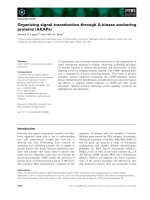
graph of the data from a typical inhibition experiment is shown in Fig. 2. The
amount of radioligand bound is plotted vs the concentration of the unlabeled
ligand (on a logarithmic scale). The bottom of the curve defines the amount of

nonspecific binding. The IC
50
value is defined as the concentration of an unla-
beled drug required to inhibit specific binding of the radioligand by 50%. The
K
i
is then calculated from the IC
50
.
Radioligand-Binding Assays 3
Fig. 2. Typical inhibition experiment. In this simulation the specific binding is
900 cpm and the IC
50
(the concentration of drug that inhibits 50% of the specific bind-
ing) is 10 nM.
1.3. Kinetic Experiments
Kinetic experiments have two main purposes. The first is to establish an
incubation time that is sufficient to ensure that steady state (commonly called
equilibrium) has been reached. The second is to determine the forward (k
+1
)
and reverse (k
–1
) rate constants. The ratio of these constants provides an inde-
pendent estimate of the K
d
(k
–1
/k
+1

). If the amounts of receptor and radioligand
are held constant and the time varied, then kinetic data are obtained from which
forward and reverse rate constants can be estimated. A graph of the data from
a typical association kinetic experiment is shown in Fig. 3. Initially the rate of
the forward reaction exceeds the rate of the reverse reaction. After approx
25 min the amount of specific binding no longer increases and thus steady state
has been reached. From these data, the k
+1
can be calculated.
For a dissociation experiment, the radioligand is first allowed to bind to the
receptor and then the dissociation of the radioligand from the receptor is mon-
itored by the decrease in specific binding (Fig. 4). The rebinding of the radio-
ligand to the receptor is prevented by the addition of a high concentration of a
nonradioactive drug that binds to the receptor and thus blocks the receptor bind-
ing site, or by “infinite” dilution which reduces the free concentration of the
radioligand. Dissociation follows first-order kinetics and thus k
–1
is equal to
the t
1
⁄2 for dissociation divided by 0.693 (natural logarithm of 2).
4 Bylund et al.
Fig. 3. Typical association experiment. In this simulation steady state is reached
after approx 25 min and lasts until the end of the experiment (42 min).
1.4. Assays in Intact Cells
Although isolated membranes are by far the most common preparation used
for radioligand-binding assays, for some purposes it is preferable to use intact
cells. The most obvious advantage of assays with intact cells is that the recep-
tor is being studied in its native environment in the cell. A related advantage of
intact cell assays is that the binding properties of the receptor can be assessed

in the same preparation and under essentially the same conditions as the func-
tional responses mediated by the receptor are measured. This allows a more
direct comparison of the receptor binding properties with a wide variety of
physiological responses following activation or inhibition of the receptor. Intact
cell assays may also be advantageous when a large number of different cell
samples need to be studied, because intact cell assays eliminate the need to
lyse cells and isolate membranes prior to assay. For example, intact cell assays
have proven very useful for preliminary screening of cell colonies following
transfection with cDNA for various G-protein-coupled receptors, thus allowing
rapid identification of clones for amplification and further analysis.
Most of the considerations that make intact cell assays advantageous in cer-
tain cases also represent limitations of intact cell assays in other cases. For
example, intact cell assays allow studies under physiological conditions, but
they make it much more difficult to vary or control the assay conditions to
Radioligand-Binding Assays 5
Fig. 4. Typical dissociation experiment. In this simulation the t
1
⁄
2
(the time at which
the specific binding has decreased by 50%) is 5 min.
identify factors that modulate receptor binding. Radioligand uptake into cells by
various transport processes can occur with intact cells, and care must be taken
to ensure that radioligand association with intact cells is due to binding rather
than uptake. The occurrence of adaptive regulatory changes in receptor number,
localization, and binding properties during the course of binding assays with
intact cells can also present a serious complication (1). Finally, intact cells have
membrane permeability barriers that are not present in isolated membrane
preparations, and therefore the lipid solubility and membrane permeability of
both the radioligand and the competing ligands must be considered in assays

with intact cells. Lipophilic (“lipid-loving”) ligands generally cross all cell
membranes easily and thus have access to both cell surface receptors and those
in intracellular compartments such as endosomes. In contrast, hydrophilic
(“water-loving”) ligands are relatively impermeable to the plasma membrane,
and thus these ligands label only cell surface receptors. Although these prop-
erties can complicate assays with intact cells, they also provide the basis for
important radioligand-binding-based assays for receptor internalization, as dis-
cussed previously (1).
2. Materials
The information given in this section is specifically for assays with mem-
brane preparations. Additional information for intact cell assays is given in
Subheading 3.4.
1. A radioligand appropriate for the receptor being studied (see Note 1). For mem-
brane saturation experiments, add the appropriate volume of radioligand into
550 µL of 5 mM HCl in a glass test tube. Thoroughly mix and add 200 µL of this
solution to 300 µL of 5 mM HCl. Prepare successive dilutions in the same manner
by adding 200 µL of each dilution to 300 µL of 5 mM HCl to obtain the next
lower dilution until six concentrations of radioligand have been prepared. This
dilution strategy gives a 100-fold range of radioligand concentrations. Other dilu-
tion strategies will give different ranges as indicated in Table 1 (see Note 2). For
membrane inhibition and kinetic experiments, only a single concentration of radi-
oligand is needed (see Note 3).
2. A source of receptor, either membranes or intact cells. The standard procedure for
a membrane assay is to homogenize the tissue or cells of interest in a hypotonic
buffer using either a Polytron (Brinkman) or similar homogenizer. Remarkably,
most receptors are stable at room temperature (generally for hours), although it is
wise to put the tissue on ice quickly. Homogenize about 500 mg of tissue in
approx 35 mL of wash buffer (50 mM Tris-HCl or similar buffer at pH 7.0–8.0)
using a Polytron (PT10-35 generator with PT10/TS probe) at setting 7 for 20 s
(see Note 4). The actual weight of tissue used should be recorded. Centrifuge at

20,000 rpm (48,000g) in a Sorvall RC5-B using an SS34 rotor (or similar cen-
trifuge and rotor) for 10 min at 4° C (see Note 5). Decant the supernatant, and
6 Bylund et al.
repeat the homogenization and centrifugation. The tissue preparation can either be
used immediately or stored frozen as a pellet until needed (see Note 6). Generally
protease inhibitors are not needed, but could be important in the case of certain
tissues or with certain receptors.
3. Membrane assay buffer, 25 mM at pH 7.4, such as sodium phosphate or Tris. For
a few receptors the choice of buffer is important, but for most it is not.
4. Wash buffer such as 25 mM Tris, pH 7.4. Almost any buffer at neutral pH will
serve the purpose.
5. 5 mM HCl for diluting labeled and unlabeled ligands. For many ligands, using a
slightly acidic diluent will increase stability and decrease binding to test tubes.
6. Appropriate unlabeled ligands in solution.
7. 0.1 M NaOH for samples to be used to assay protein.
8. Polypropylene test tubes, 12 × 75 mm (assay tubes).
9. Borosilicate glass test tubes, 12 × 75 mm (dilution tubes).
10. Glass fiber filters (GF/A circles and GF/B strips).
11. Filtration manifold.
12. Scintillation vials if using a
3
H-radioligand, or test tubes if using a
125
I-radioligand.
13. Scintillation cocktail (if using a
3
H-radioligand).
3. Methods
3.1. Saturation Experiment (Membrane Assay)
1. Resuspend washed membrane preparation in distilled water by homogenization.

2. Add three 20-µL aliquots of the tissue suspension to 80 µL of 0.1 M NaOH for
estimating protein concentration.
Radioligand-Binding Assays 7
Table 1
Dilution of Radioligand for Saturation
Experiments
µL of radioligand 250.41 200.41 150.41
µL of diluent 250.41 300.41 350.41
Dilution number Relative concentration
1 100.78 100.41 10011.
2 150.78 14011 13011.
3 125.78 11611. 119.01
4 112.58116.41112.71
5 116.28112.61110.81
6 113.18111.01110.24
7 111.68110.41
8 110.78
9 110.39
3. Add sufficient ice-cold assay buffer to the membrane suspension to give the
appropriate final concentration (see Note 7).
4. Set up a rack of 24 polypropylene incubation tubes, 6 tubes across and 4 tubes deep.
If using a
125
I-ligand add two additional test tubes to each of the 6 sets of tubes (for
the determination of total added radioactivity). If using a
3
H-ligand, prepare a set of
12 uncapped scintillation vials with GF/A glass fiber filter discs (see Note 8).
5. To the 12 tubes on the last two rows, add 10 µL of a high concentration of an
unlabeled ligand to determine nonspecific binding (see Note 9).

6. To all 24 tubes add 970 µL of the membrane preparation. Because this is a par-
ticulate suspension, it should be stirred slowly while aliquots are being removed.
7. Starting with the most dilute radioligand solution, add 20 µL to the columns of
four tubes, and mix each tube. Also add 20 µL of the radioligand solution to the
two filter papers on the scintillation vials (if using a
3
H-radioligand) or two test
tubes (if using a
125
I-ligand) for the determination of total added radioactivity.
8. Mix all the tubes again and incubate (usually at room temperature) for 45 min.
Assuming that the system is at steady state, the exact time is not critical. The
tubes may need to be rearranged to be compatible with the specific style of fil-
tration manifold used.
9. Filter the contents of the tubes and wash the filters twice with 5 mL of wash
buffer. Depending on the rate of dissociation of the radioligand from the receptor,
it may be important to use ice-cold wash buffer.
10. Place the filters into scintillation vials, add 5 mL of scintillation cocktail and cap
if using a
3
H-radioligand; or into test tubes if a using
125
I-ligand.
11. Shake the scintillation vials gently for 1 h (or let stand at room temperature over-
night) and then count in a liquid scintillation counter (if using a
3
H-radioligand); or
count in a gamma counter (if using a
125
I-ligand) (see Note 10).

3.1.1. Calculation of Results from a Saturation Experiment
Data from a sample saturation experiment are shown in Table 2. (The meth-
ods and calculations for the sample competition and inhibition experiments are
also available in an interactive format at http://www
.unmc.edu/Pharmacology/
receptortutorial/.)
1. Total binding and nonspecific binding can be plotted vs total added as shown in
Fig. 5. for the sample experiment. This plot allows one to detect data points that
may be problematic. Note that the nonspecific binding is linear (except possibly
at the lowest concentrations), and that the specific binding saturates (is relatively
constant) at high radioligand concentrations.
2. Specific binding is determined by subtracting nonspecific binding from total bind-
ing at each concentration of radioligand (see Table 2).
3. The cpm values are converted to picomolar values using a conversion factor that
accounts for specific activity for the radioligand, the counting efficiency of the
particular scintillation counter used, and the conversion factor 2.2 × 10
12
dpm/Ci.
For this experiment the counting efficiency was 0.36 and the specific radioactiv-
8 Bylund et al.
ity of the radioligand was 60 Ci/mmol, and the factor for converting cpm to dpm
is 0.0210 as shown:
cpm dpm Ci mmol 1000 mL
—— × ———– × —————— × —— × ———– ×
mL 0.36 cpm 2.2 × 10
12
dpm 60 Ci L
1 mol 10
12
pmoL 2.10 × 10

–2
pmol
————– × ————– = —————–—–
1000 mmol mol L
The results of this conversion for the sample experiment are shown in Table 3.
Radioligand-Binding Assays 9
Table 2
Results of a Sample Saturation Experiment
a
in cpm
Total added Total bound Nonspecifically bound Specifically bound
b
(cpm) (cpm) (cpm) (cpm)
11,2360 208 18 190
11,5601 394 25 369
114,491 597 46 551
132,011 782 88 694
182,520 984 189 795
199,248 1210 416 794
a
[
3
H]RX821002 binding to human α
2A
-adrenergic receptors in HT-29 cells.
b
The amount of radioligand specifically bound was also determined by subtracting the non-
specifically bound from the total bound.
Fig. 5. Total binding and nonspecific binding vs total added for a sample experiment
from Table 2.

4. The free concentration of radioligand is calculated by subtracting specifically
bound from total added as shown in Table 3.
5. The data are then plotted as bound vs free as shown in Fig. 6 for the typical sat-
uration experiment (see Note 11). The K
d
and B
max
values are generally calcu-
lated by nonlinear regression of the specific binding vs the concentration of
radioligand using a computer program as such Prism (GraphPad, San Diego, CA)
or a variety of other software packages using the following equation:
B
max
× F
B = ———–
K
d
+ F
where B is the amount of radioligand specifically bound, F is the free radio-
ligand concentration, B
max
is the radioligand concentration required to saturate all
of the binding sites, and K
d
is the dissociation constant for the radioligand at these
receptors.
6. The B
max
values are dependent on the concentration of protein in the assay. Note
that the results are given in pM units. To convert the B

max
values to pmol/mg of
protein, the pM values are converted to pmol/mL and divided by the protein con-
centration (mg/mL) used in the assay. In this example the protein concentration is
0.072 mg/assay tube and the B
max
value is calculated as shown:
17.7 pmol 1 L 1 mL 0.246 pmol
———— × ———— × 1 mL × ———— = ————–
L 1000 mL 0.072 mg mg
7. To visualize the results better and to detect potential problems, the data are fre-
quently transformed (as shown in Table 3) and viewed as a Rosenthal plot (2) in
10 Bylund et al.
Table 3
Results of Sample Saturation Experiment Given in Table 2
Converted to pM Units
Total added Specifically bound Free
(pM)(pM)(pM) Bound/free
4.37 3.99 46 0.0867
8.27 7.74 110 0.0704
12.5 11.5 292 0.0394
16.4 14.5 658 0.0220
20.7 16.7 1720 0.00971
25.4 16.7 4020 0.00415
the form of bound/free vs bound as shown in Fig. 7 (see Note 12). The equation
for the line is:
Bound 1 B
max
——— = – —– Bound + —–
Free K

d
K
d
Radioligand-Binding Assays 11
Fig. 6. Saturation curve for data from a sample saturation experiment. Specifically
bound (pM units) from Table 3 is plotted vs the free (pM) concentration of the radio-
ligand. The line was drawn using nonlinear regression analysis for one-site binding
using the Prism computer program (GraphPad, San Diego, CA).
Fig. 7. Rosenthal plot for sample saturation experiment. The bound/free vs bound
data from Table 3 are plotted to obtain the Rosenthal plot.
In this plot, the intercept with the x-axis (abscissa) is the B
max
and the K
d
is the
negative reciprocal of the slope (see Note 13). The data points fall close to a
straight line, indicating a single class of binding sites.
3.2. Inhibition Experiment
1. Prepare a 1 mM solution of the inhibitor(s) in 5 mM HCl (or other diluent as
appropriate). Dilute 0.3 mL of this solution with 0.7 mL of 5 mM HCl to give
a 0.3 mM solution. Prepare 100 µM,10µM,1 µM, 100 nM, 10 nM,1 nM, and
0.1 nM solutions by sequentially diluting 100 µL of the previous solution (i.e.,
10-fold higher concentration) with 900 µL of 5 mM HCl. Similarly, prepare
30 µM,3 µM, 300 nM, and 30 nM solutions from the 0.3 mM solution (see Note 14).
2. If using a
3
H-ligand, prepare two uncapped scintillation vials with GF/A glass
fiber filter discs (see Note 8).
3. Set up 24 assay tubes in two rows of 12. Add 10 µL of 5 mM HCl (or other dilu-
ent) to the first pair of tubes. Add 10 µL of the appropriate dilution (concentra-

tion) of the inhibitor to the other pairs of tubes, starting with the lowest
concentration (see Note 15).
4. Add 970 µL of the membrane preparation to each of the 24 tubes.
5. Add 20 µL of radioligand to each of the tubes and mix to start the incubation.
Pipet 20 µL of the radioligand solution directly onto duplicate GF/A glass fiber
filter discs (if using a
3
H-radioligand) or into two test tubes (if using a
125
I-ligand)
to determine the total added radioactivity.
6. Mix all of the tubes again and incubate at room temperature for 45 min. Assum-
ing that the system is at steady state, the exact time is not critical.
7. Filter the contents of the tubes and wash the filters twice with 5 mL of ice-cold
wash buffer. The tubes may need to be rearranged to be compatible with the
specific style of filtration manifold used.
8. Place the filters into scintillation vials, add 5 mL of scintillation cocktail, and
cap (if using a
3
H-radioligand); or place the filters into test tubes (if using a
125
I-ligand).
9. Shake the scintillation vials gently for 1 h (or let stand at room temperature over-
night) and then count in a liquid scintillation counter (if using a
3
H-radioligand)
or in a gamma counter (if using a
125
I-ligand) (see Note 10).
3.2.1. Calculation of Results from an Inhibition Experiment

The calculation of K
i
values from inhibition experiments is relatively
straightforward. The inhibition data are simply fit to a sigmoidal curve with
the logarithm of concentration of the inhibitor on the abscissa, and the IC
50
value (the concentration of the inhibitor that inhibits 50% of the specific bind-
ing) determined using a Hill slope of 1.
Top – Bottomn
Y = Bottom + ——————————–
1 + 10
(X – LogIC
50
)(Hill slope)
12 Bylund et al.
Top and bottom refer to the concentration of bound radioligand at the top and
bottom of the curve. Y is the amount of radioactive ligand bound at each con-
centration of inhibitor X. The K
i
value is calculated from the IC
50
value using
the equation
IC
50
K
i
= ———
1 + ——
where F is the free radioligand concentration and K

d
is the affinity of the radi-
oligand. This is often called the Cheng–Prusoff equation (3) (see Note 16).
Thus, if the radioligand is present at its K
d
concentration, then the K
i
is one half
of the IC
50
.
If more than one binding site is suspected, the Hill slope can be allowed to
vary or the equation for two-site binding can be used.
Span × Fraction 1 Span × (1 – Fraction 1)
Y = ———–———— + ———–——————
1 + 10
X – Log IC
50
1
1 + 10
X – LogIC
50
2
In this equation span refers to the difference between the top and bottom of the
curve, fraction 1 is the amount of radioligand bound to the high-affinity site,
and log IC
50
1
and IC
50

2
refer to the inhibition of binding to high- and low-
affinity sites, respectively. An F-test can be used to determine whether the data
better fit a one-site or a two-site model (see Example 1).
These analyses are illustrated with the data from a sample experiment given
in Table 4.
1. The data are plotted as bound (cpm or pM units) vs logarithm of the inhibitor
concentration as shown for the sample experiment in Fig. 8. The bottom of the
curve plateaus at the same bound value as obtained with norepinephrine, indicat-
ing that prazosin is likely binding to the same sites as norepinephrine.
2. The solid curve was obtained using a nonlinear regression analysis of a one-site
competition equation using the Prism computer program (GraphPad, San Diego,
CA). The data were also fit to a sigmoid curve using nonlinear regression analy-
sis with a variable Hill slope (n
H
) as is indicated by the dashed line. As is shown
in Table 5, the results of the two analyses are essentially identical because the n
H
is not different from unity. As a rough approximation, n
H
values need to be < 0.8
to be significantly different from 1.0 and suggest more complex binding.
3. Similarly the data can also be fit to a two-site competition equation. The results of
this fit are shown in Fig. 8 and Table 5 (see Note 17).
4. An F-test is used to determine whether the data fit a one- or two-site equation better.
The F-test for the sample experiment is shown in Example 1. The two-site fit was
not significantly better than the one-site fit; thus the curve for the one-site fit was
chosen, and the IC
50
values from the one-site fit were used to calculate the K

i
values.
Radioligand-Binding Assays 13
F
K
d
5. The K
i
is calculated using the Cheng–Prusoff equation (3). For the sample exper-
iment, the concentration of radioligand was 0.75 nM, the K
d
was 0.89 nM, and the
log of IC
50
was –8.04 (9.08 nM). Putting these numbers into the Cheng–Prusoff
equation gives a K
i
of 4.9 nM).
IC
50
9.08nM
K
i
= ——–— = —–—–—— = 4.9 nM
1 + — 1 + —–——
14 Bylund et al.
F
K
d
0.75 nM

0.89nM
The F-test is used to compare the one-site and the two-site models. The basic
steps are:
1. Analyze the data for a one- and two-site fit using nonlinear regression
analysis.
2. Apply the sum of the squares and degrees of freedom to the equation for
an F-test:
F = (SS1 – SS2) / (DF1 – DF2)
F = ———————————
F = SS2 / DF2
where SS1 = sum of squares for one-site fit
where SS2 = sum of squares for two-site fit
where DF1 = degrees of freedom for one-site fit
where DF2 = degrees of freedom for two-site fit
3. Determine the p value from an F-table of statistics.
4. The p value answers the question: if model 1 (one-site fit) is correct, what
is the chance that you would randomly obtain data that fits model 2 (two-
site fit) much better?
5. If p is low, you conclude that model 2 (two-site fit) is significantly better
than model 1.
6. The calculation for the sample saturation experiment:
F = (25,467 – 14,394) / (8 – 6)
F = ——–————————
F = 14,394 / 6
F = F = 2.308
F = p = 0.1806
7. Because p > 0.05, the two-site model does not give a significantly better
fit and the one-site model is accepted.
Example 1.
F-test for comparison of fit of data from sample competition experiment

to a one- vs two-site fit.
6. Frequently the total binding for different receptor preparations or different unla-
beled ligands is different, so inhibition curves are often normalized so that the
percent inhibition can be more easily compared as shown in Fig. 9.
3.3. Kinetic Experiments
3.3.1. Dissociation Experiment
1. If using a
3
H-ligand, prepare two uncapped scintillation vials with GF/A glass
fiber filter discs (see Note 8).
2. Set up 48 assay tubes in four rows of 12. To the 12 tubes on the last two rows, add
10 µL of a high concentration of an unlabeled ligand to determine nonspecific
binding (see Note 9).
3. Add 970 µL of the membrane preparation to each of the 48 tubes.
4. Add 20 µL of radioligand to all tubes and mix to start the incubation. The reac-
tion is allowed to proceed until steady-state conditions are reached (45 min). At
Radioligand-Binding Assays 15
Table 4
Data from a Sample Inhibition Experiment
a
Prazosin – Log of prazosin Average bound Specifically bound
b
% Specifically
concentration (nM) concentration (M) (cpm) (cpm) bound
c
(0)
d
–12 1395 1314 100
0.3 –9.52 1292 1211 92.2
1–91256 1175 89.4

3 –8.52 958 877 66.7
10 –8 730 649 19.4
30 –7.52 417 336 25.6
100 –7 198 117 8.90
300 –6.52 126 45 3.43
1000 –6 116 35 2.67
3000 –5.52 82 1 0.076
10,000 –5 81 0 0
NE
e
92
a
Prazosin inhibition of [
3
H]RX821002 binding to α
2B
-adrenergic receptors transfected into CHO
cells with K
d
= 0.89 nM. The concentration of radioligand used in all the tubes was 0.75 nM.
b
The amount of radioligand specifically bound was also determined by subtracting the amount
bound in the presence of the highest concentration of prazosin.
c
The data were normalized by dividing specifically bound by amount of radioligand bound in the
absence of prazosin.
d
Although the first inhibitor concentration is zero, to run the nonlinear regression program a
number needs to be used. Routinely a concentration that is at least one log unit lower than the
lowest unlabeled drug concentration is used.

e
Norepinephrine (NE) was used at a concentration of 0.3 mM to determine the extent of non-
specific binding in this experiment.
appropriate time intervals, add a high concentration (50 times the IC
50
) of unla-
beled ligand to tubes 2–12 in each row to start the dissociation reaction. The first
tube in each row is used to determine binding at zero time at the start of the dis-
sociation reaction. All incubations will be terminated at the same time by filtra-
tion. Thus, the unlabeled ligand is added at various times, for example 1, 2, 4, 7,
10, 15, 20, 25, 30, 40, and 60 min before filtration. Also pipet 20 µL of the radi-
16 Bylund et al.
Fig. 8. Plot of inhibition data for a sample experiment. The data from Table 4 are
plotted as bound (cpm) vs the prazosin concentration (in log molar units). The solid
curve was obtained using a one-site model. Determination of the IC
50
is based on the
middle of the curve (725 cpm bound) and not half of the binding in the absence of pra-
zosin (697 cpm bound). The dashed curve is from both a two-site analysis and an
analysis of a sigmoid equation with a variable Hill slope (the curves are essentially
identical for these data).
Table 5
Results of Analysis of the Sample Inhibition Experiment Presented in Table 4
Parameter Single-site fit Variable Hill slope fit Two-site fit
Bottom of curve 1193 cpm 1174 cpm 1180 cpm
Top of curve 1356 cpm 1390 cpm 1389 cpm
Log IC
50
–8.04 –8.06 –8.62
IC

50
–9.08 nM –8.72 nM –2.39 nM
Log IC
50
, second site –7.76
IC
50
, second site 17.2 nM
Fraction, second site 0.64
The curves for these data are shown in Fig. 8.
oligand solution directly onto duplicate GF/A glass fiber filter discs (if using a
3
H-radioligand) or two test tubes (if using a
125
I-ligand) to estimate the total added
radioactivity (see Note 18).
5. Filter the contents of the tubes and wash the filters twice with 5 mL of ice-cold
wash buffer. The tubes may need to be rearranged to be compatible with the spe-
cific style of filtration manifold used.
6. Place the filters into scintillation vials, add 5 mL of scintillation cocktail, and cap
(if using a
3
H-radioligand); or place the filters into test tubes (if a using
125
I-ligand).
7. Shake the scintillation vials gently for 1 h (or let stand at room temperature over-
night) and then count in a liquid scintillation counter (if using a
3
H-radioligand),
or count in a gamma counter (if using a

125
I-ligand) (see Note 10).
3.3.2. Calculation of Results from a Dissociation Experiment
Data from a sample experiment are given in Table 6. Note that in a dissoci-
ation experiment time zero is the time at which the unlabeled ligand is added
to the assay tube. The time course for the dissociation experiment then becomes
the time between when the unlabeled ligand is added to the assay tube and the
time when the samples are filtered.
1. Nonspecific binding is subtracted from total binding at each time point. Specific
binding from a sample experiment is presented in Table 6.
2. The data are plotted as bound vs dissociation time. The data from the sample
experiment are plotted in Fig. 10.
Radioligand-Binding Assays 17
Fig. 9. Plot of normalized data for the sample inhibition experiment. The normalized
data from Table 4 are plotted as a function of the log of the inhibitor concentration.
This plot is more useful when multiple data sets are being compared.
3. The data are analyzed using a nonlinear regression program using the equation for
exponential decay:
Y = Span * e
–k*X
+ Nonspecific binding
In a dissociation experiment span refers to specific binding and k is k
–1
.
Analysis of the data for the sample experiment using a one-site exponential decay
analysis and the Prism computer program (GraphPad, San Diego, CA) gives a k
–1
of 0.117 min
–1
.

3.3.3. Association Experiments
1. If using a
3
H-ligand, prepare two uncapped scintillation vials with GF/A glass
fiber filter discs (see Note 8).
2. Set up 48 assay tubes in four rows of 12. To the 12 tubes on the last two rows add
10 µL of a high concentration of an unlabeled ligand to determine nonspecific
binding (see Note 9).
3. Add 970 µL of the membrane preparation to each of the 48 tubes.
4. At appropriate time intervals, add 20 µL radioligand to all of the tubes and mix.
All incubations will be terminated at the same time by filtration. Thus, the
radioactivity is added at, for example, 1, 2, 4, 7, 10, 15, 20, 25, 30, 40, 50, and
60 min before filtration. Also pipet 20 µL of the radioligand solution directly onto
duplicate GF/A glass fiber filter discs (if using a
3
H-radioligand) or two test tubes
(if using a
125
I-ligand) to estimate the total added radioactivity.
18 Bylund et al.
Table 6
Data from a Sample Dissociation
Experiment
a
Time Specifically bound
(min) (cpm)
0 577
1 490
2 460
3 400

4 360
6 280
8 215
10 165
12 140
a
[
3
H]DHA was incubated with guinea pig cerebral
cortex membranes for 20 min to label β-adrenergic
receptors. Isoproterenol (2 µM ) was added at time
zero. Samples were filtered at the times indicated.
5. Filter the contents of the tubes and wash the filters twice with 5 mL of ice-cold
wash buffer. The tubes may need to be rearranged to be compatible with the
specific style of filtration manifold used.
6. Place the filters into scintillation vials, add 5 mL of scintillation cocktail, and
cap (if using a
3
H-radioligand); or place the filters into test tubes (if using a
125
I-ligand).
7. Shake the scintillation vials gently for 1 h (or let stand at room temperature over-
night) and then count in a liquid scintillation counter (if using a
3
H-radioligand);
or count in a gamma counter (if using a
125
I-ligand) (see Note 10).
3.3.4. Calculation of Results from an Association Experiment
1. Nonspecific binding is subtracted from total binding at each time point to give

specific binding. The data from a sample experiment are given in Table 7.
2. Amount bound is plotted vs time as shown in Fig. 11 for the sample association
experiment.
3. The data are analyzed using a nonlinear regression analysis of the equation for an
exponential association curve:
Y = Y
max
(1 – e
–K
ob
t)
The rate constant (k
ob
) obtained is a combination of k
1
and k
–1
and will vary with
the concentration of radioligand (F) added to the assay according to the follow-
ing equation:
k
ob
= k
1
F + k
–1
Radioligand-Binding Assays 19
Fig. 10. Plot of data from the sample dissociation experiment given in Table 6. The
line was drawn using the nonlinear regression equation for one-phase exponential decay
using the Prism computer program (GraphPad, San Diego, CA).

k
–1
can be determined using a separate dissociation experiment as described
above. Then, k
1
can be determined using the following rearrangement of the above
equation:
k
ob
– k
–1
k
1
= ——–—
F
Nonlinear regression analysis of the sample association data (Table 7; Fig. 11)
gave a k
ob
= 0.187 min
–1
at a radioligand concentration of 0.36 nM. The dissociation
rate constant determined from the experiment described above was 0.117 min
–1
.
The association rate constant for the sample experiment thus becomes:
0.187 min
–1
– 0.117 min
–1
k

1
= ——————————– = 0.194 min
–1
nM
–1
0.36 nM
An alternate way to determine k
1
is to perform the association experiment at var-
ious concentrations of radioactive ligand. The k
ob
determined from these associa-
tion experiments can then be plotted vs the concentration of radioligand (F). The
y-intercept is the k
–1
and the slope of the line is k
1
.
4. K
d
is determined by dividing k
–1
/k
1
. For the sample experiment:
0.117 min
–1
K
d
= —————–—— = 0.60 nM

0.194 min
–1
nM
–1
20 Bylund et al.
Table 7
Data from a Sample Association
Experiment
a
Time Specifically bound
(min) (cpm)
1.5 0.0
0.0 170
2.5 285
4.0 380
6.0 475
8.0 560
10.0 610
13.0 655
16.0 680
20.0 710
a
Radioligand binding of 0.36 nM [
3
H]DHA to
guinea pig cerebral cortex.
3.4. Sample Protocol for a Saturation Experiment With Monolayer Cells
Assays with intact cells in suspension are quite similar to assays with mem-
branes. The manipulations required for assays with monolayer cells are more
involved, however, and thus a detailed protocol for monolayer cells is presented

below (see Note 19). The protocol described is for an eight-point saturation
experiment with triplicate determinations for both total and nonspecific binding.
The protocol assays the cells in sets of six (three total binding and three non-
specific binding), because this is a convenient number to manipulate within a
1-min time frame (1 every 10 s). Accordingly the cells are plated on 6-well
plates, and the plates are treated at 5-min intervals.
1. Grow cells to near confluence on eight 6-well plates in 2 mL of growth medium
per well (see Note 20).
2. Prepare 7.5 mL of 4-(2-hydroxyethyl)piperazine-1-ethanesulfonic acid (HEPES)-
buffered serum-free growth medium (see Note 21) containing each of the eight
concentrations of radioligand, labeled as A–H. Transfer 3.5 mL of these solutions
to each of two polypropylene tubes with a large enough diameter to allow easy
use of a 1-mL pipettor tip (see Note 22). To one of each pair of tubes (for total
binding), add 35 µL of the vehicle for the agent used to define nonspecific bind-
ing and label as “AT-HT.” To the other (for nonspecific binding), add 35 µL of
100×-concentrated solution of the agent used to define nonspecific binding and
Radioligand-Binding Assays 21
Fig. 11. Plot of data for sample association experiment presented in Table 7. The
line was drawn using the nonlinear regression equation for exponential association
using the Prism computer program (GraphPad, San Diego, CA).
label as “AN-HN.” Place these tubes in a 37°C water bath to reach physiological
temperature (see Note 23).
3. Place a beaker with approx 300 mL of HEPES-buffered serum-free growth
medium in the 37°C water bath as well, to be used as preincubation wash
medium. This same medium can be used as postincubation wash buffer, although
in some cases it is beneficial for the postincubation wash buffer to contain a drug
to reduce nonspecific binding (see Note 23).
4. Prepare a Pasteur pipet connected by Tygon tubing to a vacuum flask connected
to a vacuum pump or vacuum line to use for aspirating medium from dishes.
5. A detailed time course for a 60-min assay in which a single investigator can con-

duct the entire assay is presented below, with times presented in minutes. All solu-
tion additions are done with a Pipetman or similar hand-held adjustable pipettor.
These solutions should be gently added against the inside wall of the dish, not
directly onto the monolayers, to avoid loss of cells from the dish due to the mul-
tiple medium changes.
a. Initiation of binding:
t = 0 min: At 10-s intervals, aspirate the growth medium and add 2 mL of
37°C preincubation wash buffer to the six wells of the first
plate. This step is to wash away serum and bicarbonate and
switch the cells to the medium used as assay buffer.
t = 1 min: At 10-s intervals, aspirate the wash buffer from the plate and
add 1 mL of AT solution to the top three wells and 1 mL of AN
solution to the bottom three wells. By starting the T wells
before the N wells, it is not necessary to change pipet tips
between the total and nonspecific binding solutions. However,
the tip must be changed before the next concentration of total
binding solution is added to the next set of dishes.
t = 2 min: Transfer the plate to a 37°C non-CO
2
incubator for the 60-min
binding time.
t = 5, 6, 7 min: Repeat the above steps for the second plate, using the BT and
BN solutions.
t = 10, 11, 12, 15, Repeat the above steps for each of the remaining six concentra-
16, 17 min, etc.: tions of radioligand.
b. Termination of binding:
t = 60 min: At 10-s intervals, aspirate the binding medium and add 2 mL of
37°C postincubation wash buffer (see Note 24) to the three AT
wells and then the 3 AN wells. This step is to stop the binding
reaction and wash away unbound radioligand.

t = 61 min: Repeat the preceding step for a second wash of the first plate.
t = 62 min: At 10-s intervals, aspirate the wash buffer and add 1 mL of 0.2 M
NaOH to each of the six wells. Set the plate aside (see Note 25).
t = 65, 66, 67 min: Repeat the above steps for the BT and BN plates.
t = 70, 71, 72, Repeat the above steps for each of the remaining six plates.
75, 76, 77 min, etc.:
22 Bylund et al.
Transfer and quantitation of bound radioactivity: after the binding and wash steps
are completed for all eight plates, transfer the dissolved cells and the associated
radioactivity to vials for scintillation counting or to tubes for gamma counting,
depending on the radioligand used (see Note 26).
6. Only minimal modifications to this protocol are needed for competition rather
than saturation assays.
7. Kinetic assays of association and dissociation become somewhat more compli-
cated with intact cells grown in monolayer culture. Because each well must be
started and stopped individually, careful planning of the time points is required. In
general, the longer time points are started first and stopped last to complete the
entire experiment in the shortest possible time. An example of sample timing that
allows a single investigator to conduct a time course experiment with time points
at 2, 5, 10, 20, 40, and 60 min is presented below.
t = 0, 1, 2 min: Start the binding reaction for the 60-min plate.
t = 5, 6, 7 min: Start the binding reaction for the 40-min plate.
t = 10, 11, 12 min: Start the binding reaction for the 20-min plate.
t = 15, 16, 17 min: Start the binding reaction for the 10-min plate.
t = 25, 26, 27 min: Stop the reaction for the 10-min plate.
t = 30, 31, 32 min: Stop the reaction for the 20-min plate.
t = 35, 36, 37 min: Start the binding reaction for the 5-min plate.
t = 40, 41, 42 min: Stop the reaction for the 5-min plate.
t = 45, 46, 47 min: Stop the reaction for the 40-min plate.
t = 50, 51 min: Start the reaction for the 2-min plate; this plate will be

stopped immediately.
t = 52, 53, 54 min: Stop the reaction for the 2-min plate.
t = 65, 66, 67 min: Stop the reaction for the 60-min plate.
4. Notes
1. The decision as to which radioligand to use is based both on the characteristics of
the radioligand and on the specific scientific questions being asked. The important
characteristics to be considered include the radioisotope (
3
H or
125
I), the extent of
nonspecific binding, the selectivity and affinity of the radioligand for the receptor,
and whether the radioligand is an agonist or an antagonist.
The advantages of
3
H over
125
I as a radioisotope include that the radioligand is
chemically unaltered and thus biologically indistinguishable from the unlabeled
compound, and that it has a longer half-life (12 yr vs 60 d). Because of their short
half-lives, iodinated radioligands are usually purchased or prepared every 4–6 wk,
whereas
3
H-ligands can often be used for several months or even longer. An
advantage of the iodinated radioligands is their higher specific activity (up to 2200 Ci/
mmol vs 30–100 Ci/mmol for
3
H-ligands), which makes them particularly useful
if the density of receptors is low or if the amount of tissue is small. It is easier and
less expensive to use iodinated ligands, because scintillation cocktail is not

needed, thus eliminating purchasing and disposal costs associated with scintilla-
tion cocktail.
Radioligand-Binding Assays 23
Each radioligand has a unique pharmacological profile. The radioligand should
bind selectively to the receptor type or subtypes of interest under the assay condi-
tions used. Although no radioligand is completely selective for any given receptor
or receptor subtype, some are better than others. If, for example, several subtypes
of a receptor are present in a given tissue, and if the intent is to label all the sub-
types, then a subtype nonselective radioligand that has nearly equal affinity for all
three of the subtypes would be chosen. By contrast, if only a single subtype is of
primary interest, then a radioligand having higher affinity for that particular subtype
as compared to the other subtypes would be the preferred radioligand.
Usually the higher the affinity the better, because a lower concentration of
the radioligand can be used in the assay, which results in a lower level of non-
specific binding. Furthermore, a higher affinity usually means a slower rate of
dissociation, which provides for a more convenient assay.
Agonist radioligands may label only a portion of the total receptor population
(the high-affinity state for G-protein-coupled receptors), whereas antagonist lig-
ands generally label all receptors. On the other hand, an agonist radioligand may
more accurately reflect receptor alterations of biological significance, because it is
agonists that activate the receptor.
Usually the radioligand with the lowest nonspecific (or nonreceptor) binding
is best. An assay is considered barely adequate if 50% of the total binding is
specific; 70% is good and 90% is excellent.
Most radioligands are stored in an aqueous solution that often contains an
organic solvent such as ethanol. These solutions should be stored cold but not
frozen, because freezing of the solution tends to concentrate the radioligand
locally and increase its radiolytic destruction.
2. At least six concentrations of radioligand should be used with an equal number above
and below the anticipated K

d
value. Thus, the amount of stock radioligand used will
depend on the K
d
of the radioligand for the receptor type and subtype assayed.
The amount of radioligand prepared in this manner is sufficient for three saturation
experiments. We routinely use 5 mM HCl to dilute the radioactivity because we
have found that it reduces the nonspecific binding of many radioligands to the
dilution tubes and help to ensure ligand stability. This may not be necessary for all
radioligands. The small amount (20 µL) of dilute HCl (5 mM) carried over to the
1.0-mL assay in 25 mM buffer does not alter the pH of the assay. Because the
amount of specific binding approaches the B
max
asymptotically, the specific bind-
ing will never actually reach the B
max
and thus true saturation will be never be
achieved. Furthermore, the use of very high radioligand concentration is usually
limited by the associated high level of nonspecific binding and by cost. In practice,
for an assay that conforms to a single site, it is sufficient if the highest concentra-
tion gives specific binding of >90% of the B
max
and that the Rosenthal line is linear.
3. The radioligand concentration used in inhibition experiment should be less than its
K
d
value. For kinetic experiments to establish steady state, the lowest practical
concentration should be used. For experiments to calculate K
d
from k

+1
and k
–1
,a
concentration near the K
d
usually works well.
24 Bylund et al.