digital simulation in electrochemistry 3ed 2005 - britz
Bạn đang xem bản rút gọn của tài liệu. Xem và tải ngay bản đầy đủ của tài liệu tại đây (2.38 MB, 337 trang )
Lecture Notes in Physics
Editorial Board
R. Beig, Wien, Austria
W. B eig l b
¨
ock, Heidelberg, Germany
W. Domcke, Garching, Germany
B G. Englert, Singapore
U. Frisch, Nice, France
P. H
¨
anggi, Augsburg, Germany
G. Hasinger, Garching, Germany
K. Hepp, Z
¨
urich, Switzerland
W. Hillebrandt, Garching, Germany
D. Imboden, Z
¨
urich, Switzerland
R. L. Jaffe, Cambridge, MA, USA
R. Lipowsky, Golm, Germany
H. v. L
¨
ohneysen, Karlsruhe, Germany
I. Ojima, Kyoto, Japan
D. Sornette, Nice, France, and Los Angeles, CA, USA
S. Theisen, Golm, Germany
W. Weise, Garching, Germany
J. Wess, M
¨
unchen, Germany
J. Zittartz, K
¨
oln, Germany
The Editorial Policy for Monographs
The series Lecture Notes in Physics reports new developments in physical research and
teaching - quickly, informally, and at a high level. The type of material considered for
publication includes monographs presenting original research or new angles in a classical
field. The timeliness of a manuscript is more important than its form, which may be
preliminary or tentative. Manuscripts should be reasonably self-contained. They will often
present not only results of the author(s) but also related work by other people and will
provide sufficient motivation, examples, and applications.
Acceptance
The manuscripts or a detailed description thereof should be submitted either to one of
the series editors or to the managing editor. The proposal is then carefully refereed. A
final decision concerning publication can often only be made on the basis of the complete
manuscript, but otherwise the editors will try to make a preliminary decision as definite
as they can on the basis of the available information.
Contractual Aspects
Authors receive jointly 30 complimentary copies of their book. No royalty is paid on Lecture
Notes in Physics volumes. But authors are entitled to purchase directly from Springer other
books from Springer (excluding Hager and Landolt-Börnstein) at a 33
1
3
% discount off the
list price. Resale of such copies or of free copies is not permitted. Commitment to publish
is made by a letter of interest rather than by signing a formal contract. Springer secures
the copyright for each volume.
Manuscript Submission
Manuscripts should be no less than 100 and preferably no more than 400 pages in length.
Final manuscripts should be in English. They should include a table of contents and an
informative introduction accessible also to readers not particularly familiar with the topic
treated. Authors are free to use the material in other publications. However, if extensive
use is made elsewhere, the publisher should be informed. As a special service, we offer
free of charge L
A
T
E
X macro packages to format the text according to Springer’s quality
requirements. We strongly recommend authors to make use of this offer, as the result
will be a book of considerably improved technical quality. The books are hardbound, and
quality paper appropriate to the needs of the author(s) is used. Publication time is about ten
weeks. More than twenty years of experience guarantee authors the best possible service.
LNP Homepage (springerlink.com)
On the LNP homepage you will find:
−The LNP online archive. It contains the full texts (PDF) of all volumes published since
2000. Abstracts, table of contents and prefaces are accessible free of charge to everyone.
Information about the availability of printed volumes can be obtained.
−The subscription information. The online archive is free of charge to all subscribers of
the printed volumes.
−The editorial contacts, with respect to both scientific and technical matters.
−Theauthor’s/editor’sinstructions.
Dieter Britz
Digital Simulation
in Electrochemistry
Third Completely Revised and Extended Edition
With Supplementary Electronic Material
123
Author
Dieter Britz
Kemisk Institut
˚
Arhus Universitet
8000
˚
Arhus C
Denmark
Email:
Dieter Britz, DigitalSimulationinElectrochemistry,
Lect. Notes Phys. 666 (Springer, Berlin Heidelberg 2005), DOI 10.1007/b97996
Library of Congress Control Number: 2005920592
ISSN 0075-8450
ISBN 3-540-23979-0 3rd ed. Springer Berlin Heidelberg New York
ISBN 3-540-18979-3 2nd ed. Springer-Verlag Berlin Heidelberg New York
ISBN 3-540-10564-6 1st ed. published as Vol. 23 in Lectur e No tes in Chemistry
Springer-Verlag Berlin Heidelberg New York
This work is subject to copyright. All rights are reserved, whether the whole or part
of the material is concerned, specifically the rights of translation, reprinting, reuse of
illustrations, recitation, broadcasting, reproduction on microfilm or in any other way, and
storage in data banks. Duplication of this publication or parts thereof is permitted only
under the provisions of the German Copyright Law of September 9, 1965, in its current
version, and permission for use must always be obtained from Springer. Violations are
liable to prosecution under the German Copyright Law.
Springer is a part of Springer Science+Business Media
springeronline.com
© Springer-Verlag Berlin Heidelberg 2005
Printed in Germany
The use of general descriptive names, registered names, trademarks, etc. in this publication
does not imply, even in the absence of a specific statement, that such names are exempt
from the relevant protective laws and regulations and therefore free for general use.
Typesetting: by the authors and TechBooks using a Springer L
A
T
E
X macro package
Cover design: design & production,Heidelberg
Printed on acid-free paper
2/3141/jl-543210
This book is dedicated to H. H. Bauer, teacher and friend
Preface
This book is an extensive revision of the earlier 2nd Edition with the same
title, of 1988. The book has been rewritten in, I hope, a much more didac-
tic manner. Subjects such as discretisations or methods for solving ordinary
differential equations are prepared carefully in early chapters, and assumed
in later chapters, so that there is clearer focus on the methods for partial
differential equations. There are many new examples, and all programs are
in Fortran 90/95, which allows a much clearer programming style than earlier
Fortran versions.
In the years since the 2nd Edition, much has happened in electrochemical
digital simulation. Problems that ten years ago seemed insurmountable have
been solved, such as the thin reaction layer formed by very fast homogeneous
reactions, or sets of coupled reactions. Two-dimensional simulations are now
commonplace, and with the help of unequal intervals, conformal maps and
sparse matrix methods, these too can be solved within a reasonable time.
Techniques have been developed that make simulation much more efficient,
so that accurate results can be achieved in a short computing time. Stable
higher-order methods have been adapted to the electrochemical context.
The book is accompanied (on the webpage www.springerlink.com/
openurl.asp?genre=issue&issn=1616-6361&volume=666) by a number of ex-
ample procedures and programs, all in Fortran 90/95. These have all been
verified as far as possible. While some errors might remain, they are hopefully
very few.
I have a debt of gratitude to a number of people who have checked the
manuscript or discussed problems with me. My wife Sandra polished my Eng-
lish style and helped with some of the mathematics, and Tom Koch Sven-
nesen checked many of the mathematical equations. Others I have consulted
for advice of various kinds are Professor Dr. Bertel Kastening, Drs. Leslaw
Bieniasz, Ole Østerby, J¨org Strutwolf and Thomas Britz. I thank the various
editors at Springer for their support and patience. If I have left anybody out,
I apologize. As is customary to say (and true), any errors remaining in the
book cannot be blamed on anybody but myself.
˚
Arhus, Dieter Britz
February 2005
Contents
1 Introduction 1
2 Basic Equations 5
2.1 General . . . . . . . . . . . . . . . . . . . . . . . . . . . . . . . . . . . . . . . . . . . . . . . 5
2.2 Some Mathematics: Transport Equations . . . . . . . . . . . . . . . . . . 6
2.2.1 Diffusion . . . . . . . . . . . . . . . . . . . . . . . . . . . . . . . . . . . . . . . . 6
2.2.2 Diffusion Current . . . . . . . . . . . . . . . . . . . . . . . . . . . . . . . . . 7
2.2.3 Convection . . . . . . . . . . . . . . . . . . . . . . . . . . . . . . . . . . . . . . 8
2.2.4 Migration . . . . . . . . . . . . . . . . . . . . . . . . . . . . . . . . . . . . . . . 9
2.2.5 Total Transport Equation . . . . . . . . . . . . . . . . . . . . . . . . . 10
2.2.6 Homogeneous Kinetics . . . . . . . . . . . . . . . . . . . . . . . . . . . . 10
2.2.7 Heterogeneous Kinetics . . . . . . . . . . . . . . . . . . . . . . . . . . . 12
2.3 Normalisation – Making the Variables Dimensionless . . . . . . . . 12
2.4 Some Model Systems and Their Normalisations . . . . . . . . . . . . 14
2.4.1 Potential Steps . . . . . . . . . . . . . . . . . . . . . . . . . . . . . . . . . . . 14
2.4.2 Constant Current . . . . . . . . . . . . . . . . . . . . . . . . . . . . . . . . 24
2.4.3 Linear Sweep Voltammetry (LSV) . . . . . . . . . . . . . . . . . . 25
2.5 Adsorption Kinetics . . . . . . . . . . . . . . . . . . . . . . . . . . . . . . . . . . . . 28
3 Approximations to Derivatives 33
3.1 Approximation Order . . . . . . . . . . . . . . . . . . . . . . . . . . . . . . . . . . . 33
3.2 Two-Point First Derivative Approximations . . . . . . . . . . . . . . . . 34
3.3 Multi-Point First Derivative Approximations . . . . . . . . . . . . . . . 36
3.4 The Current Approximation . . . . . . . . . . . . . . . . . . . . . . . . . . . . . 38
3.5 The Current Approximation Function G 39
3.6 High-Order Compact (Hermitian) Current Approximation . . . 39
3.7 Second Derivative Approximations . . . . . . . . . . . . . . . . . . . . . . . . 43
3.8 Derivatives on Unevenly Spaced Points . . . . . . . . . . . . . . . . . . . . 44
3.8.1 Error Orders . . . . . . . . . . . . . . . . . . . . . . . . . . . . . . . . . . . . . 47
3.8.2 A Special Case . . . . . . . . . . . . . . . . . . . . . . . . . . . . . . . . . . . 48
3.8.3 Current Approximation . . . . . . . . . . . . . . . . . . . . . . . . . . . 48
3.8.4 A Specific Approximation . . . . . . . . . . . . . . . . . . . . . . . . . 48
X Contents
4 Ordinary Differential Equations 51
4.1 An Example ode 51
4.2 Local andGlobal Errors 52
4.3 WhatDistinguishestheMethods 52
4.4 EulerMethod 52
4.5 Runge-Kutta, RK . . . . . . . . . . . . . . . . . . . . . . . . . . . . . . . . . . . . . . 54
4.6 BackwardsImplicit, BI 56
4.7 Trapeziumor MidpointMethod 56
4.8 Backward Differentiation Formula, BDF . . . . . . . . . . . . . . . . . . . 57
4.8.1 Starting BDF . . . . . . . . . . . . . . . . . . . . . . . . . . . . . . . . . . . . 58
4.9 Extrapolation . . . . . . . . . . . . . . . . . . . . . . . . . . . . . . . . . . . . . . . . . . 61
4.10 Kimble & White, KW . . . . . . . . . . . . . . . . . . . . . . . . . . . . . . . . . . . 62
4.10.1 Using KW as a Start for BDF . . . . . . . . . . . . . . . . . . . . . 64
4.11 Systems of ode s 65
4.12 Rosenbrock Methods . . . . . . . . . . . . . . . . . . . . . . . . . . . . . . . . . . . . 67
4.12.1 Application to a Simple Example ODE . . . . . . . . . . . . . . 70
4.12.2 Error Estimates . . . . . . . . . . . . . . . . . . . . . . . . . . . . . . . . . . 71
5 The Explicit Method 73
5.1 The Discretisation . . . . . . . . . . . . . . . . . . . . . . . . . . . . . . . . . . . . . . 73
5.2 Practicalities . . . . . . . . . . . . . . . . . . . . . . . . . . . . . . . . . . . . . . . . . . . 74
5.3 Chronoamperometry and -Potentiometry . . . . . . . . . . . . . . . . . . 76
5.4 Homogeneous Chemical Reactions (hcr) 77
5.4.1 The Reaction Layer. . . . . . . . . . . . . . . . . . . . . . . . . . . . . . . 79
5.5 Linear Sweep Voltammetry . . . . . . . . . . . . . . . . . . . . . . . . . . . . . . 80
5.5.1 Boundary Condition Handling . . . . . . . . . . . . . . . . . . . . . 81
6 Boundary Conditions 85
6.1 Classification of Boundary Conditions . . . . . . . . . . . . . . . . . . . . . 85
6.2 Single Species: The u-v Device 86
6.2.1 Dirichlet Condition . . . . . . . . . . . . . . . . . . . . . . . . . . . . . . . 86
6.2.2 Derivative Boundary Conditions . . . . . . . . . . . . . . . . . . . . 86
6.3 TwoSpecies 90
6.3.1 Two-Point Derivative Cases . . . . . . . . . . . . . . . . . . . . . . . . 93
6.4 Two Species with Coupled Reactions. U-V 94
6.5 BruteForce 100
6.6 A General Formalism . . . . . . . . . . . . . . . . . . . . . . . . . . . . . . . . . . . 101
7 Unequal Intervals 103
7.1 Transformation . . . . . . . . . . . . . . . . . . . . . . . . . . . . . . . . . . . . . . . . . 104
7.1.1 Discretising the Transformed Equation . . . . . . . . . . . . . . 105
7.1.2 The Choice of Parameters . . . . . . . . . . . . . . . . . . . . . . . . . 107
7.2 Direct Application of an Arbitrary Grid . . . . . . . . . . . . . . . . . . . 107
7.2.1 Choice of Parameters . . . . . . . . . . . . . . . . . . . . . . . . . . . . . 110
7.3 Concluding Remarks on Unequal Spatial Intervals . . . . . . . . . . 110
Contents XI
7.4 Unequal Time Intervals . . . . . . . . . . . . . . . . . . . . . . . . . . . . . . . . . 111
7.4.1 Implementation of Exponentially Increasing Time
Intervals 112
7.5 Adaptive IntervalChanges 112
7.5.1 Spatial Interval Adaptation . . . . . . . . . . . . . . . . . . . . . . . . 113
7.5.2 Time Interval Adaptation . . . . . . . . . . . . . . . . . . . . . . . . . 116
8 The Commonly Used Implicit Methods 119
8.1 The Laasonen MethodorBI 121
8.2 The Crank-Nicolson Method, CN . . . . . . . . . . . . . . . . . . . . . . . . . 121
8.3 Solving theImplicitSystem 122
8.4 Using Four-Point Spatial Second Derivatives . . . . . . . . . . . . . . . 124
8.5 Improvements on CN and Laasonen . . . . . . . . . . . . . . . . . . . . . . . 126
8.5.1 Damping the CN Oscillations . . . . . . . . . . . . . . . . . . . . . . 127
8.5.2 Making Laasonen More Accurate . . . . . . . . . . . . . . . . . . . 131
8.6 Homogeneous Chemical Reactions . . . . . . . . . . . . . . . . . . . . . . . . 134
8.6.1 Nonlinear Equations . . . . . . . . . . . . . . . . . . . . . . . . . . . . . . 135
8.6.2 Coupled Equations . . . . . . . . . . . . . . . . . . . . . . . . . . . . . . . 140
9 Other Methods 145
9.1 The Box Method 145
9.2 Improvements onStandardMethods 148
9.2.1 The Kimble and White Method . . . . . . . . . . . . . . . . . . . . 148
9.2.2 Multi-Point Second Spatial Derivatives . . . . . . . . . . . . . . 151
9.2.3 DuFort-Frankel . . . . . . . . . . . . . . . . . . . . . . . . . . . . . . . . . . 152
9.2.4 Saul’yev . . . . . . . . . . . . . . . . . . . . . . . . . . . . . . . . . . . . . . . . . 154
9.2.5 Hopscotch . . . . . . . . . . . . . . . . . . . . . . . . . . . . . . . . . . . . . . . 156
9.2.6 Runge-Kutta . . . . . . . . . . . . . . . . . . . . . . . . . . . . . . . . . . . . 158
9.2.7 Hermitian Methods . . . . . . . . . . . . . . . . . . . . . . . . . . . . . . . 159
9.3 Method of Lines (MOL)
and Differential Algebraic Equations (DAE) . . . . . . . . . . . . . . . 165
9.4 The Rosenbrock Method 167
9.4.1 An Example, the Birk-Perone System . . . . . . . . . . . . . . . 170
9.5 FEM,BEMandFAM(briefly) 172
9.6 Orthogonal Collocation, OC . . . . . . . . . . . . . . . . . . . . . . . . . . . . . 173
9.6.1 Current Calculation with OC . . . . . . . . . . . . . . . . . . . . . . 180
9.6.2 A Numerical Example . . . . . . . . . . . . . . . . . . . . . . . . . . . . 180
9.7 Eigenvalue-Eigenvector Method . . . . . . . . . . . . . . . . . . . . . . . . . . 182
9.8 Integral Equation Method . . . . . . . . . . . . . . . . . . . . . . . . . . . . . . . 184
9.9 The NetworkMethod 185
9.10 Treanor Method . . . . . . . . . . . . . . . . . . . . . . . . . . . . . . . . . . . . . . . . 186
9.11 Monte Carlo Method. . . . . . . . . . . . . . . . . . . . . . . . . . . . . . . . . . . . 187
XII Contents
10 Adsorption 189
10.1 Transport and Isotherm Limited Adsorption . . . . . . . . . . . . . . . 190
10.2 Adsorption Rate Limited Adsorption . . . . . . . . . . . . . . . . . . . . . . 191
11 Effects Due to Uncompensated Resistance
and Capacitance 193
11.1 Boundary Conditions . . . . . . . . . . . . . . . . . . . . . . . . . . . . . . . . . . . 195
11.1.1 An Example . . . . . . . . . . . . . . . . . . . . . . . . . . . . . . . . . . . . . 197
12 Two-Dimensional Systems 201
12.1 Theories . . . . . . . . . . . . . . . . . . . . . . . . . . . . . . . . . . . . . . . . . . . . . . . 202
12.1.1 The Ultramicrodisk Electrode, UMDE . . . . . . . . . . . . . . 202
12.1.2 Other Microelectrodes . . . . . . . . . . . . . . . . . . . . . . . . . . . . 208
12.1.3 Some Relations . . . . . . . . . . . . . . . . . . . . . . . . . . . . . . . . . . 209
12.2 Simulations . . . . . . . . . . . . . . . . . . . . . . . . . . . . . . . . . . . . . . . . . . . . 210
12.3 Simulating the UMDE . . . . . . . . . . . . . . . . . . . . . . . . . . . . . . . . . . 212
12.3.1 Direct Discretisation . . . . . . . . . . . . . . . . . . . . . . . . . . . . . . 213
12.3.2 Discretisation in the Mapped Space . . . . . . . . . . . . . . . . . 221
12.3.3 A Remark on the Boundary Conditions . . . . . . . . . . . . . 232
13 Convection 235
13.1 Some Fluid Dynamics . . . . . . . . . . . . . . . . . . . . . . . . . . . . . . . . . . . 235
13.1.1 Layer Relations . . . . . . . . . . . . . . . . . . . . . . . . . . . . . . . . . . 239
13.2 Electrodes in Flow Systems . . . . . . . . . . . . . . . . . . . . . . . . . . . . . . 239
13.3 Simulations . . . . . . . . . . . . . . . . . . . . . . . . . . . . . . . . . . . . . . . . . . . . 240
13.4 A Simple Example: The Band Electrode
in a Channel Flow . . . . . . . . . . . . . . . . . . . . . . . . . . . . . . . . . . . . . . 241
13.5 Normalisations . . . . . . . . . . . . . . . . . . . . . . . . . . . . . . . . . . . . . . . . . 242
14 Performance 247
14.1 Convergence . . . . . . . . . . . . . . . . . . . . . . . . . . . . . . . . . . . . . . . . . . . 247
14.2 Consistency . . . . . . . . . . . . . . . . . . . . . . . . . . . . . . . . . . . . . . . . . . . . 250
14.3 Stability . . . . . . . . . . . . . . . . . . . . . . . . . . . . . . . . . . . . . . . . . . . . . . . 251
14.3.1 Heuristic Method . . . . . . . . . . . . . . . . . . . . . . . . . . . . . . . . . 251
14.3.2 Von Neumann Stability Analysis . . . . . . . . . . . . . . . . . . . 252
14.3.3 Matrix Stability Analysis . . . . . . . . . . . . . . . . . . . . . . . . . . 254
14.3.4 Some Special Cases . . . . . . . . . . . . . . . . . . . . . . . . . . . . . . . 260
14.4 The Stability Function . . . . . . . . . . . . . . . . . . . . . . . . . . . . . . . . . . 261
14.5 Accuracy Order . . . . . . . . . . . . . . . . . . . . . . . . . . . . . . . . . . . . . . . . 263
14.5.1 Order Determination . . . . . . . . . . . . . . . . . . . . . . . . . . . . . 264
14.6 Accuracy, Efficiency and Choice . . . . . . . . . . . . . . . . . . . . . . . . . . 266
14.7 Summary of Methods . . . . . . . . . . . . . . . . . . . . . . . . . . . . . . . . . . . 270
Contents XIII
15 Programming 273
15.1 Language and Style . . . . . . . . . . . . . . . . . . . . . . . . . . . . . . . . . . . . . 273
15.2 Debugging . . . . . . . . . . . . . . . . . . . . . . . . . . . . . . . . . . . . . . . . . . . . . 274
15.3 Libraries . . . . . . . . . . . . . . . . . . . . . . . . . . . . . . . . . . . . . . . . . . . . . . 275
16 Simulation Packages 277
A Tables and Formulae 281
A.1 First Derivative Approximations . . . . . . . . . . . . . . . . . . . . . . . . . . 281
A.2 Current Approximations. . . . . . . . . . . . . . . . . . . . . . . . . . . . . . . . . 282
A.3 Second Derivative Approximations . . . . . . . . . . . . . . . . . . . . . . . . 282
A.4 Unequal Intervals 282
A.4.1 First Derivatives . . . . . . . . . . . . . . . . . . . . . . . . . . . . . . . . . 283
A.4.2 Second Derivatives . . . . . . . . . . . . . . . . . . . . . . . . . . . . . . . 284
A.5 Jacobi Roots for Orthogonal Collocation . . . . . . . . . . . . . . . . . . 285
A.6 RosenbrockConstants 285
B Some Mathematical Proofs 289
B.1 Consistency of the Sequential Method . . . . . . . . . . . . . . . . . . . . . 289
B.2 TheFeldberg StartforBDF 290
B.3 Similarity of the Feldberg Expansion
and Transformation Functions . . . . . . . . . . . . . . . . . . . . . . . . . . . 295
C Procedure and Program Examples 299
C.1 ExampleModules 299
C.2 Procedures . . . . . . . . . . . . . . . . . . . . . . . . . . . . . . . . . . . . . . . . . . . . 301
C.2.1 Procedures for Unequal Intervals . . . . . . . . . . . . . . . . . . . 302
C.2.2 JCOBI . . . . . . . . . . . . . . . . . . . . . . . . . . . . . . . . . . . . . . . . . . 304
C.3 ExamplePrograms 304
References 313
Index 331
1 Introduction
This book is about the application of digital simulation to electrochemical
problems. What is digital simulation? The term “simulation” came into wide
use with the advent of analog computers, which could produce electrical
signals that followed mathematical functions to describe or model a given
physical system. When digital computers became common, people began to
do these simulations digitally and called this digital simulation. What sort
of systems do we simulate in electrochemistry? Most commonly they are
electrochemical transport problems that we find difficult to solve, in all but
a few model systems – when things get more complicated, as they do in real
electrochemical cells, problems may not be solvable algebraically, yet we still
want answers.
Most commonly, the basic equation we need to solve is the diffusion equa-
tion, relating concentration c to time t and distance x from the electrode
surface, given the diffusion coefficient D:
∂c
∂t
= D
∂
2
c
∂x
2
. (1.1)
This is Fick’s second diffusion equation [242], an adaptation to diffusion of
the heat transfer equation of Fourier [253]. Technically, it is a second-order
parabolic partial differential equation (pde ). In fact, it will mostly be only the
skeleton of the actual equation one needs to solve; there will usually be such
complications as convection (solution moving) and chemical reactions taking
place in the solution, which will cause concentration changes in addition to
diffusion itself. Numerical solution may then be the only way we can get
numbers from such equations – hence digital simulation.
The numerical technique most commonly employed in digital simulation
is (broadly speaking) that of finite differences and this is much older than
the digital computer. It dates back at least to 1911 [468] (Richardson). In
1928, Courant, Friedrichs and Lewy [182] described what we now take to be
the essentials of the method; Emmons [218] wrote a detailed description of
finite difference methods in 1944, applied to several different equation types.
There is no shortage of mathematical texts on the subject: see, for example,
Lapidus and Pinder [350] and Smith [514], two excellent books out of a large
number.
Dieter Britz: Digital Simulation in Electrochemistry, Lect. Notes Phys. 666,1–4 (2005)
www.springerlink.com
c
Springer-Verlag Berlin Heidelberg 2005
2 1 Introduction
It should not be imagined that the technique became used only when dig-
ital computers appeared; engineers certainly used it long before that time,
and were not afraid to spend hours with pencil and paper. Emmons [218]
casually mentions that one fluid flow problem took him 36 hours! Not surpris-
ingly, it was during this early pre-computer era that much of the theoretical
groundwork was laid and refinements worked out to make the work easier –
those early stalwarts wanted their answers as quickly as possible, and they
wanted them correct the first time through.
Electrochemical digital simulation is almost synonymous with Stephen
Feldberg, who wrote his first paper on it in 1964 [234]. It is not always
remembered that Randles [460] used the technique much earlier (in 1948),
to solve the linear sweep problem. He did not have a computer and did the
arithmetic by hand. The most widely quoted electrochemical literature source
is Feldberg’s chapter in Electroanalytical Chemistry [229], which describes
what will here be called the “box” method. Feldberg is rightly regarded as
the pioneer of digital simulation in electrochemistry, and is still prominent
in developments in the field today. This has also meant that the box method
has become standard practice among electrochemists, while what will here
be called the “point” method is more or less standard elsewhere. Having
experimented with both, the present author favours the point method for the
ease with which one arrives at the discrete form of one’s equations, especially
when the differential equation is complicated.
A brief description will now be given of the essentials of the simulation
technique. Assume (1.1) above. We wish to obtain concentration values at a
given time over a range of distances from the electrode. We divide space (the
x coordinate) into small intervals of length h and time t into small time steps
δt. Both x and t can then be expressed as multiples of h and δt,usingi as
the index along x and j as that for t,sothat
x
i
= ih (1.2)
and
t
j
= jδt . (1.3)
Figure 1.1 shows the resulting grid of points. At each drawn point, there
is a value of c. The digital simulation method now consists of developing
rows of c values along x, (usually) one t-step at a time. Let us focus on
the three filled-circle points c
i−1
, c
i
and c
i+1
at time t
j
. One of the various
techniques to be described will compute from these three known points a new
concentration value c
i
= c
i
(t =(j +1)δt) (empty circle) at x
i
for the next
time value t
j+1
, by expressing (1.1) in discrete form:
c
i
− c
i
δt
=
D
h
2
(c
i−1
− 2c
i
+ c
i+1
) . (1.4)
1 Introduction 3
Fig. 1.1. Discrete sample point grid
The only unknown in this equation is c
i
and it can be explicitly calculated.
Having obtained c
i
, we move on to the next x point and compute c
for it, etc.,
until all c values for that row, for the next time value, have been computed.
In the remainder of the book, the various schemes for calculating new
points will often be graphically described by isolating the marked circles seen
in Fig. 1.1; in this case, the scheme would be represented by the following
diagram
This follows the convention seen in such texts as Lapidus and Pinder [350]
(who call it the “computational molecule”, which will also be the name for
it in this book). It is very convenient, as one can see at a glance what a
particular scheme does. The filled points are known points while the empty
circles are those to be calculated.
Several problems will become apparent. The first one is that of the method
used to arrive at (1.4); this will be dealt with later. There is, in fact, a
multiplicity of methods and expressions used. The second problem is the
concentration value at x = 0; there is no x
−1
point, as would be needed
for i = 1. The value of c
0
is a boundary value, and must be determined by
some other method. Another boundary value is the last x point we treat.
How far out into the diffusion space should (need) we go? Usually, we know
good approximations for concentrations at some sufficiently large distance
from the electrode (e.g., either “bulk” concentration, or zero for a species
generated at the electrode), and we have pretty good criteria for the distance
we need to go out to. Another boundary lies at the row for t = 0: this is the
row of starting values. Again, these are supplied by information other than
4 1 Introduction
the diffusional process we are simulating (but, for a given method, can be
a problem, as will be seen in a later chapter). Boundary problems are dealt
with in Chap. 6. They are, in fact, a large part of what this book is about,
or what makes it specific to electrochemistry. The discrete diffusion equation
we have just gone through could just as well apply to heat transfer or any
other diffusion transport problems.
Throughout the book, the following symbol convention will be used: di-
mensioned quantities like concentration, distance or time will be given lower-
case symbols (c, x, t, etc.) and their non-dimensional equivalents will be given
the corresponding upper-case symbols (C, X, T , etc.), with a few unavoidable
exceptions.
2 Basic Equations
2.1 General
In this chapter, we present most of the equations that apply to the systems
and processes to be dealt with later. Most of these are expressed as equations
of concentration dynamics, that is, concentration of one or more solution
species as a function of time, as well as other variables, in the form of differ-
ential equations. Fundamentally, these are transport (diffusion-, convection-
and migration-) equations but may be complicated by chemical processes
occurring heterogeneously (i.e. at the electrode surface – electrochemical re-
action) or homogeneously (in the solution bulk – chemical reaction). The
transport components are all included in the general Nernst-Planck equation
(see also Bard and Faulkner 2001) for the flux J
j
of species j
J
j
= −D
j
∇C
j
−
z
j
F
RT
D
j
C
j
∇φ + C
j
v (2.1)
in which J
j
is the molar flux per unit area of species j at the given point in
space, D
j
the species’ diffusion coefficient, C
j
its concentration, z
j
its charge,
F, R and T have their usual meanings, φ is the potential and v the fluid
velocity vector of the surrounding solution (medium). The symbol ∇ denotes
the differentiation operator and it is directional in 3-D space. This equation
is a more general form of Fick’s first diffusion equation, which contains only
the first term on the right-hand side, the diffusion term. The second term
on that side is the migration term and the last, the convection term. These
will now be discussed individually. At the end of the chapter, we go through
some models and electrode geometries, and present some known analytical
solutions, as well as dimensionless forms of the equations. There is no term
in the equation to take account of changes due to chemical reactions taking
place in the solution, since these do not give rise to a flux of substance. Such
terms come in later, in the equations relating concentration changes with
time to the above components (see (2.15) and Sect. 2.2.6).
Dieter Britz: Digital Simulation in Electrochemistry, Lect. Notes Phys. 666,5–32 (2005)
www.springerlink.com
c
Springer-Verlag Berlin Heidelberg 2005
6 2 Basic Equations
2.2 Some Mathematics: Transport Equations
2.2.1 Diffusion
For a good text on diffusion, see the monograph of Crank [183]. Consider
Fig. 2.1. We imagine a chosen coordinate direction x in a solution volume
containing a dissolved substance at concentration c, which may be different
at different points – i.e., there may be concentration gradients in the solution.
We consider a very small area δA on a plane normal to the x-axis. Fick’s first
equation now says that the net flow of solute (flux f
x
, in mol s
−1
) crossing
the area is proportional to the negative of the concentration gradient at the
plane, in the x-direction
f
x
=
dn
dt
= −δA D
dc
dx
(2.2)
with D a proportionality constant called the diffusion coefficient and n the
number of moles. This can easily be understood upon a moment’s thought;
statistically, diffusion is a steady spreading out of randomly moving particles.
If there is no concentration gradient, there will be an equal number per unit
time moving backward and forward across the area δA, and thus no net flow.
If there is a gradient, there will be correspondingly more particles going in one
direction (down the gradient) and a net increase in concentration on the lower
side will result. Equation (2.2) is of precisely the same form as the first heat
flow equation of Fourier [253]; Fick’s contribution [242] lay in realising the
analogy between temperature and concentration, heat and mass (or number
of particles). The quantity D has units m
2
s
−1
(SI) or cm
2
s
−1
(cgs).
Fig. 2.1. Diffusion across a small area
Equation (2.2) is the only equation needed when using the box method and
this is sometimes cited as an advantage. It brings one close to the microscopic
system, as we shall see, and has – in theory – great flexibility in cases where
the diffusion volume has an awkward geometry. In practice, however, most
geometries encountered will be – or can be simplified to – one of but a few
2.2 Some Mathematics: Transport Equations 7
standard forms such as cartesian, cylindrical or spherical – for which the full
diffusion equation has been established (see, e.g., Crank [183]). In cartesian
coordinates this equation, Fick’s second diffusion equation, in its most general
form, is
∂c
∂t
= D
x
∂
2
c
∂x
2
+ D
y
∂
2
c
∂y
2
s + D
z
∂
2
c
∂z
2
. (2.3)
This expresses the rate of change of concentration with time at given coordi-
nates (t, x, y, z) in terms of second space derivatives and three different diffu-
sion coefficients. It is theoretically possible for D to be direction-dependent
(in anisotropic media) but for a solute in solution, it is equal in all directions
and usually the same everywhere, so (2.3) simplifies to
∂c
∂t
= D
∂
2
c
∂x
2
+
∂
2
c
∂y
2
+
∂
2
c
∂z
2
, (2.4)
that is, the usual three-dimensional form. Even this is rather rarely applied –
we always try to reduce the number of dimensions, preferably to one, giving
∂c
∂t
= D
∂
2
c
∂x
2
. (2.5)
If the geometry of the system is cylindrical, it is convenient to switch to
cylindrical coordinates: x along the cylinder, r the radial distance from the
axis and θ the angle. In most cases, concentration is independent of the angle
and the diffusion equation is then
∂c
∂t
= D
∂
2
c
∂x
2
+
∂
2
c
∂r
2
+
1
r
∂c
∂r
. (2.6)
Often there is no gradient along x (the axis), so only r remains
∂c
∂t
= D
∂
2
c
∂r
2
+
1
r
∂c
∂r
. (2.7)
For a spherical system, assuming no concentration gradients other than away
from the centre (radially), the equation becomes
∂c
∂t
= D
∂
2
c
∂r
2
+
2
r
∂c
∂r
. (2.8)
2.2.2 Diffusion Current
Equation (2.2) gives the flux in mol s
−1
of material as the result of a concen-
tration gradient. If there is such a gradient normal to an electrode/electrolyte
interface, then there is a flux of material at the electrode and this takes place
via the electron transfer. An electroactive species diffuses to the electrode,
8 2 Basic Equations
takes part in the electron transfer and becomes a new species. The electrical
current i flowing is then equal to the molar flux multiplied by the number of
electrons transferred for each molecule or ion (2.2), and the Faraday constant
i = nF AD
∂c
∂x
x=0
(2.9)
for a reduction current. The flux and the current are thus, in a sense, syn-
onymous and will, in fact, profitably be expressed simply in terms of the
concentration gradient itself or its dimensionless equivalent, to be discussed
later (Sect. 2.3).
2.2.3 Convection
If we cannot arrange for our solution to be (practically) stagnant during
our experiment, then we must include convective terms in the equations.
Figure 2.2 shows a plot of concentration against the x-coordinate at a given
instant. Let x
1
be a fixed point along x, with concentration c
1
at some time
t, and let the solution be moving forward along x with velocity v
x
, so that
after a small time interval δt, concentration c
2
(previously at x
2
) has moved
to x
1
by the distance δx.Ifδt and δx are chosen sufficiently small, we may
consider the line PQ as straight and we have, for the change δc at x
1
δc = −δx
dc
dx
(2.10)
Dividing by δt, taking v
x
= δx/δt and going to the infinitesimal limit, we get
for the x-term
∂c
∂t
= −v
x
∂c
∂x
. (2.11)
If there is convection in all three directions, this expands to
∂c
∂t
= −v
x
∂c
∂x
− v
y
∂c
∂y
− v
z
∂c
∂z
. (2.12)
Fig. 2.2. Convection
2.2 Some Mathematics: Transport Equations 9
This treatment ignores the diffusional processes taking place simultaneously;
the two transport terms are additive in the limit.
Convection terms commonly crop up with the dropping mercury elec-
trode, rotating disk electrodes and in what has become known as hydrody-
namic voltammetry, where the electrolyte is made to flow past an electrode
in some reproducible way (e.g. the impinging jet, channel and tubular flows,
vibrating electrodes, etc). This is discussed in Chap. 13.
2.2.4 Migration
Migration is included here more or less for completeness – the electrochemist
is usually able to eliminate this transport term (and will do so for practical
reasons as well). If our species is charged, that is, it is an ion, then it may
experience electrical forces due to potential fields. This will be significant
in solutions of ionic electroactive species, not containing a sufficiently large
excess of inert electrolyte.
In general (see Vetter [559]), for an electroactive cation with charge +z
A
and anion with charge −z
B
, an inert electrolyte with the same two charges
on its ions, and with r the concentration ratio electrolyte/electroactive ion,
we have the rather awkward equation
i
i
0
=
1+
z
A
z
B
(1 + r)
1 −
r
1+r
p
(2.13)
where
p =
1+
z
A
z
B
−1
(2.14)
and i
0
is the pure diffusion current, without migration effects. To illustrate,
let us take |z
A
| = |z
B
| = 1. Then i/i
0
=2forr = 0 (no inert electrolyte),
1.17 for r =1,1.02 for r = 10 and 1.002 for r = 100. For very accurate
studies, then, inert electrolyte should be in excess by a factor of 100 or more,
and this will be assumed in the remainder of the book.
There is one situation in which migration can have an appreciable effect,
even in the presence of excess inert electrolyte. For the measurement of very
fast reactions, one must resort to techniques involving very small diffusion
layers (see Sect. 2.4.1 for the definition) – either by taking measurements
at very short times or forcing the layer thickness down by some means. If
that thickness becomes comparable in magnitude with that of the diffuse
double layer, and the electroactive species is charged, then migration will
play a part in the transport to and from the electrode. The effect has been
clearly explained elsewhere [83]. A rough calculation for a planar electrode in
a stagnant solution, assuming the thickness of the diffuse double layer to be
of the order of 10
−9
m and the diffusion coefficient of the electroactive species
to be 10
−12
m
2
s
−1
(which is rather slow) shows that migration effects are
expected during the first µs or so. The situation, then, is rather extreme and
10 2 Basic Equations
we leave it to the specialist to handle it. Recently, this has been discussed [513]
in the context of ultramicroelectrodes, where this may need to be investigated
further.
2.2.5 Total Transport Equation
This section serves merely to emphasise that for a given cell system, the full
transport equation is the sum of those for diffusion, convection and migration.
We might write, quite generally,
∂c
∂t
=
∂c
∂t
diff
+
∂c
∂t
conv
+
∂c
∂t
migr
(2.15)
with the “diff” term as defined by one of the (2.3)–(2.8), the “conv” term
by (2.11) and “migr” related to (2.13). At any one instant, these terms are
simply additive. Digitally, we can “freeze” the instant and evaluate the sum
of the separate terms. There may be non-transport terms to add as well, such
as kinetic terms, to be discussed next.
2.2.6 Homogeneous Kinetics
Homogeneous reactions are chemical reactions not directly dependent upon
the electrode/electrolyte interface, taking place somewhere within the elec-
trolyte (or, in principle, the metal) phase. These lead to changes in con-
centration of reactants and/or products and can have marked effects on the
dynamics of electrochemical processes. They also render the dynamic equa-
tions much more difficult to solve and it is here that digital simulation sees
much of its use. Whereas analytical solutions for kinetic complications are
difficult to obtain, the corresponding discrete expressions are obtained sim-
ply by extending the diffusion equation by an extra, kinetic term (although
practical problems arise, see Chaps. 5, 9). The actual form of this depends
upon the sort of chemistry taking place. In the simplest case, met with in
flash photolysis, we have a single substance generated by the flash, then de-
caying in solution by a first- or second-order reaction; this is represented by
equations of the form
∂c
∂t
= −k
1
c (2.16)
or
∂c
∂t
= −2k
2
c
2
(2.17)
and these can be added to the transport terms. Very often, we have several
substances interacting chemically, as in the example of the simple electro-
chemical reaction
A + ne
−
⇔ B (2.18)
2.2 Some Mathematics: Transport Equations 11
followed by chemical decay of the product B. If this is first-order and we have
a simple one-dimensional diffusion system, we then have the two equations
(c
A
and c
B
denoting concentrations of, substances A and B, respectively; D
A
and D
B
the two respective diffusion coefficients)
∂c
A
∂t
= D
A
∂
2
c
A
∂x
2
∂c
B
∂t
= D
B
∂
2
c
B
∂x
2
− k
1
c
B
. (2.19)
There is a great variety of such reactions including dimerisation, dispropor-
tionation and catalytic reactions, both preceding and following the electro-
chemical step(s) and it is not useful to attempt to list them all here. The point
is merely to stress that they are (with greater or lesser difficulty) digitally
tractable, as will be shown in Chaps. 5 and 9.
There is one problem that makes homogeneous chemical reactions espe-
cially troublesome. Most often, a mechanism to be simulated involves species
generated at the interface, that then undergo chemical reaction in the solu-
tion. This leads to concentration profiles for these species that are confined
to a thin layer near the interface – thin, that is, compared with the diffusion
layer (see Sect. 2.4.1, the Nernst diffusion layer). This is called the reaction
layer (see [74, 257, 559]). Simulation parameters are usually chosen so as to
resolve the space within the diffusion layer and, if a given profile is much
thinner than that, the resolution of the sample point spacing might not be
sufficient. The thickness of the reaction layer depends on the nature of the
homogeneous chemical reaction. In any case, any number given for such a
thickness – as with the diffusion layer thickness – depends on how the thick-
ness is defined. Wiesner [572] first derived an expression for the reaction layer
thickness µ,
µ =
D
k
. (2.20)
(Wiesner’s expression used different symbols, but this is not important.) This
expression strictly holds only for a first-order reaction and Vetter [559] pro-
vides a more general expression. However, the above expression is sufficient
for most simulation purposes. The equation for µ holds in practice only for
rather large values of the rate constant; for small values below unity, µ be-
comes greater than the diffusion layer thickness, which will then dominate the
concentration profile. At the other end of the scale of rate constants, for very
fast reactions, µ can become very small. The largest rate constant possible
is about 10
10
s
−1
(the diffusion limit) and this leads to a µ value only about
10
−5
the thickness of the diffusion layer, so there must be some sample points
very close to the electrode. This problem has been overcome only in recent
years, first by using unequal intervals, then by the use of dynamic grids, both
of which are discussed in Chap. 7.
12 2 Basic Equations
2.2.7 Heterogeneous Kinetics
In real (as opposed to model) electrochemical cells, the net current flowing
will often be partly determined by the kinetics of electron transfer between
electrode and the electroactive species in solution. This is called heteroge-
neous kinetics, as it refers to the interface instead of the bulk solution. The
current in such cases is obtained from the Butler-Volmer expressions relating
current to electrode potential [73,74,83,257,559]. We have at an electrode the
process (2.18), with concentrations at the electrode/electrolyte interface c
A,0
and c
B,0
, respectively. We take as positive current that going into the elec-
trode, i.e., electrons leaving it, which corresponds to the reaction (2.18) going
from left to right, or a reduction. Positive or forward (reduction) current i
f
is then related to the potential E by
i
f
= nF Ac
A,0
k
0
exp
−αnF
RT
E − E
0
(2.21)
with A the electrode area, k
0
a standard heterogeneous rate constant, α the
so-called transfer coefficient which lies between 0 and 1 and E
0
the system’s
standard potential. For the reverse (oxidation) current i
b
,
i
b
= −nF Ac
B,0
k
0
exp
(1 − α)
nF
RT
E − E
0
. (2.22)
Both processes may be running simultaneously. The net current is then the
sum (i
f
+ i
b
) and this will, through (2.9), fix the concentration gradients at
the electrode in these cases.
If a reaction is very fast, it may be simpler to make the assumption of
complete reversibility or electrochemical equilibrium at the electrode, at a
given potential E. The Nernst equation then applies:
E = E
0
−
RT
nF
ln
c
B,0
c
A,0
(2.23)
or, for the purpose of computation,
c
A,0
c
B,0
=exp
nF
RT
E − E
0
. (2.24)
Just how this is applied in simulation will be seen in later chapters.
The foregoing ignores activity coefficients. If these are known, they can
be inserted. Most often they are taken as unity.
2.3 Normalisation – Making
the Variables Dimensionless
In most simulations, it will be advantageous to transform the given equation
variables into dimensionless ones. This is done by expressing them each as a