bowick, c. (1997). rf circuit design
Bạn đang xem bản rút gọn của tài liệu. Xem và tải ngay bản đầy đủ của tài liệu tại đây (17.5 MB, 178 trang )
Newnes
RF
Circuit
Design
Chris
Bdk
I
I-
RF CIRCUIT
DESIGN
Chris
Bowick
is
presently employed
as
the
Product Engineering Manager
For Headend Products with Scientific Atlanta Video Communications Division
located in Norcross, Georgia. His responsibilities include design and product
development of satellite earth station receivers and headend equipment for
use in the cable tv industry. Previously, he was associated with Rockwell Inter-
national, Collins Avionics Division, where he was a design engineer on aircraft
navigation equipment. His design experience also includes vhf receiver, hf syn-
thesizer, and broadband amplifier design, and millimeter-wave radiometer design.
Mr. Bowick holds a
BEE
degree from Georgia Tech and, in his spare time, is
working toward his
MSEE
at Georgia Tech, with emphasis on rf circuit design.
He is the author of several articles in various hobby magazines. His hobbies
include flying, ham radio
(WB4UHY
)
,
and raquetball.
RF
CIRCUIT
DESIGN
by
Chris
Bowick
Newnes
An imprint
of
Elsevier Science
Newnes is an imprint of Elsevier Science.
Copyright
0
1982 by Chris Bowick
All rights reserved
No
part of this publication may be reproduced, stored in a retrieval system, or
transmitted in any form or by any means, electronic, mechanical,
photocopying, recording, or otherwise, without the prior written permission of
the publisher.
Permissions may be sought directly from Elsevier’s Science
&
Technology
Rights Department in Oxford,
UK:
phone: (+44) 1865 843830, fax: (+44)
1865 853333, e-mail:
You
may also complete
your request on-line via the Elsevier Science homepage
(),
by selecting ‘Customer Support’ and then
‘Obtaining Permissions’.
@
This book is printed on acid-free paper.
Library
of
Congress Cataloging-in-Publication Data
Bowick, Chris.
p. cm.
RF
circuit design
/
by Chris Bowick
Originally published: Indianapolis
:
H.W. Sams, 1982
Includes bibliographical references and index.
ISBN 0-7506-9946-9 (pbk.
:
alk. paper)
1.
Radio circuits Design and construction. 2. Radio Frequency.
I.
Title.
TK6553.B633 1997 96-5 1612
621,384’12-dc20 CP
The publisher offers special discounts on bulk orders of this book
For information, please contact:
Manager of Special Sales
Elsevier Science
200 Wheeler Road
Burlington, MA
0
1803
Tel: 781-313-4700
Fax: 781-3 13-4802
For information on all Newnes publications available, contact our World
Wide Web homepage at
n
15 14 13 12 1110
Printed in the United States of America
RF
Circuit Design
is written for those who desire a practical approach to the
design of rf amplifiers, impedance matching networks, and filters. It is totally
user
oriented.
If you are an individual who has little rf circuit design experience,
you
can use this book as a catalog
of
circuits, using component values designed
for
your
application. On the other hand, if you are interested in the theory behind
the rf circuitry being designed,
you
can use the more detailed information that
is
provided for in-depth study.
An expert in the rf circuit design field will find this
book
to be an
excellent
reference
rruznual,
containing most
of
the commonly used circuit-design formulas
that are needed. However, an electrical engineering student will find this book to
be
a
valuable bridge between classroom studies and the real world. And, finally,
if
you
are an experimenter or ham, who is interested in designing your own
equipment,
RF
Circuit
Design
will provide numerous examples to guide
you
every step of the way.
Chapter
1
begins with some basics about components and how they behave
at
rf
frequencies; how capacitors become inductors, inductors become capacitors,
and wires become inductors, capacitors, and resistors. Toroids are introduced and
toroidal inductor design is covered in detail.
Chapter
2
presents
a
review
of
resonant circuits and their properties including
a discussion
of Q,
passband ripple, bandwidth, and coupling. You learn how to
design single and multiresonator circuits, at the loaded
Q
you desire. An under-
standing
of
resonant circuits naturally leads to filters and their design.
So,
Chapter
3
presents complete design procedures for multiple-pole Rutterworth, Chebyshel
and Bessel filters including low-pass, high-pass, bandpass, and bandstop designs.
LVithin minutes after reading Chapter
3,
you will be able to design multiple
pole filters to meet your specifications. Filter design was never easier.
Next, Chapter
4
covers impedance matching
of
both real and complex im-
pendances. This is done both numerically and with the aid of the Smith Chart.
hlathematics are kept to
a
bare minimum. Both high-Q and low-Q matching
networks
are covered in depth.
Transistor behavior at rf frequencies is discussed in Chapter
5.
Input im-
pedance. output impedance, feedback capacitance, and their variation over fre-
quency are outlined. Transistor data sheets are explained in detail, and
Y
and
S
parameters are introduced.
Chapter
6
details complete
cookbook
design procedures for rf small-signal
amplifiers, using both
Y
and
S
parameters. Transistor biasing, stability, impedance
matching, and neutralization techniques are covered in detail, complete with
practical examples. Constant-gain circles and stability circles, as plotted
on
a
Smith Chart, are introduced while rf amplifier design procedures for minimum
noise figure are
also
explained.
The subject of Chapter
7
is rf power amplifiers. This chapter describes the
differences between small- and large-signal amplifiers, and provides step-by-step
procedures for designing the latter. Design sections that discuss coaxial-feedline
impedance matching and broadband transformers are included.
Appendix
A
is a math tutorial on complex number manipulation
with
emphasis
on their relationship to complex impedances. This appendix is recommended
reading for those who are not familiar with complex number arithmetic. Then,
Appendix
B
presents
a
systems approach to low-noise design by examining the
Noise Figure parameter and its relationship to circuit design and total systems
design. Finally, in Appendix
C,
a
bibliography
of
technical papers and books
related to rf circuit design is given
so
that you, the reader, can further increase
your understanding
of
rf design procedures.
CHRIS
BOWICK
ACKNOWLEDGMENTS
The author wishes to gratefully acknowledge the contributions made
by
various
individuals to the completion of this project. First, and foremost, a special thanks
goes to my wife, Maureen, who not only typed the entire manuscript
at
least
twice, but also performed duties both as an editor and as the author’s principal
source of encouragement throughout the project. Needless to say, without her
help, this book would have never been completed.
Additional thanks go to the following individuals and companies for their
contributions in the form of information and data sheets: Bill Amidon and Jim
Cox of Amidon Associates, Dave Stewart of Piezo Technology, Irving Kadesh
of
Piconics, Brian Price of Indiana General, Richard Parker
of
Fair-Rite Products,
Jack Goodman of Sprague-Goodman Electronics, Phillip Smith of Analog Instru-
ments, Lothar Stern of Motorola, and Larry Ward of Microwave Associates.
To
my
wife,
Maureen, and daughter,
Zoe
. . .
CHAPTER
1
COMPONENTS
1.1
Wire
-
Resistors
-
Capacitors
-
Inductors
-
Toroids
-
Toroidal Inductor Design
-
Practical Winding Hints
CHAPTER
2
RESONANT
CIRCUITS
31
Some Definitions
-
Resonance (Lossless Components)
-
Loaded
Q
-
Insertion Loss
-
Impedance Transformation
-
Coupling
of
Resonant Circuits
CHAPTER
3
FILTER DESIGN
44
Background
-
Modem Filter Design
-
Normalization and the Low-Pass Prototype
-
Filter Types
-
Frequency and Impedance Scaling
-
High-Pass Filter Design
-
The Dual Network
-
Bandpass Filter Design
-
Summary
of
the Bandpass Filter
Design Procedure
-
Band-Rejection Filter Design
-
The Effects
of
Finite Q
CHAPTER
4
IMPEDANCE
MATCHING
66
Background
-
The L Network
-
Dealing With Complex Loads
-
Three-Element
Matching
-
Low-Q or Wideband Matching Networks
-
The Smith Chart
-
Im-
pedance Matching on the Smith Chart
-
Summary
CHAPTER
5
THE TRANSISTOR
AT
RADIO
FREQUENCIE~
99
The Transistor Equivalent Circuit
-
Y
Parameters
-
S
Parameters
-
Understanding
Rf
Transistor Data Sheets
-
Summary
CHAPTER
6
SMALL-SIGNAL
RF
AMPLIFIER
DESIGN
1x7
Transistor Biasing
-
Design Using
Y
Parameters
-
Design Using
S
Parameters
CHAPTER
7
RF
POWER AMPLIFIERS
150
Rf
Power Transistor Characteristics
-
Transistor Biasing
-
Power Amplifier Design
-
Matching to Coaxial Feedlines
-
Automatic Shutdown Circuitry
-
Broadband Trans-
formers
-
Practical Winding Hints
-
Summary
APPENDIX
A
VECTOR
ALGEBRA
APPENDIX B
NOISE
CALCULATIONS
Types
of
Noise
-
Noise Figure
-
Receiver Systems Calculations
APPENDIX
C
BIBLIOGRAPHY
Technical Papers
-
Books
INDEX
,
.
164
. .
167
. .
170
.
.
172
COMPONENTS
Components, those bits and pieces which make up
a radio frequency
(rf)
circuit, seem at times to be
taken for granted.
A
capacitor is, after all, a capacitor
-isn’t it?
A
l-megohm resistor presents an impedance
of at least
1
megohm-doesn’t it? The reactance of an
inductor always increases with frequency, right? Well,
as
we shall see later in this discussion, things aren’t
always as they seem. Capacitors at certain frequencies
may not be capacitors at all, but may look inductive,
while inductors may look like capacitors, and resistors
may tend to be a little of both.
In this chapter, we will discuss the properties of re-
sistors, capacitors, and inductors at radio frequencies
as they relate to circuit design. But, first, let’s take a
look at the most simple component of any system and
examine its problems at radio frequencies.
WIRE
Wire in an rf circuit can take many forms. Wire-
wound resistors, inductors, and axial- and radial-leaded
capacitors all use a wire of some size and length either
in their leads, or in the actual body of the component,
or both. Wire is also used in many interconnect appli-
cations in the lower rf spectrum. The behavior of
a
wire in the rf spectrum depends to a large extent on
the wire’s diameter and length. Table
1-1
lists, in the
American Wire Gauge (AWG) system, each gauge
of wire, its corresponding diameter, and other charac-
teristics
of
interest to the
rf
circuit designer. In the
AWG system, the diameter
of
a wire will roughly
double every six wire gauges. Thus,
if
the last six
EXAMPLE
1-1
Given that
the diameter
of
AWG
50
wire is
1.0
mil
(0.001 inch), what
is
the
diameter
of
AWG 14 wire?
Solution
AWG 50
=
1
mil
AWG 44
=
2
x
1
mil
=
2 mils
AWG 38
=
2
x
2 mils
=
4 mils
AWG 32
=
2
x
4 mils
=
8 mils
AWG 26
=
2
x
8
mils
=
16 mils
AWG
20
=
2
x
16
mils
=
32 mils
AWG 14
=
2
x
32 mils
=
64 mils (0.064 inch)
gauges and their corresponding diameters are mem-
orized from the chart, all other wire diameters can be
determined without the aid of a chart (Example
1-1).
Skin
Effect
A
conductor, at low frequencies, utilizes its entire
cross-sectional area
as
a transport medium for charge
carriers. As the frequency is increased, an increased
magnetic field at the center of the conductor presents
an impedance to the charge carriers, thus decreasing
the current density at the center of the conductor and
increasing the current density around its perimeter.
This increased current density near the edge
of
the
conductor is known as
skin
effect.
It
occurs in all con-
ductors including resistor leads, capacitor leads, and
inductor leads.
The depth into the conductor at which the charge-
carrier current density falls to l/e, or
37%
of its value
along the surface, is known as the
skin
depth
and is
a function of the frequency and the permeability and
conductivity of the medium. Thus, different con-
ductors, such as silver, aluminum, and copper, all have
different skin depths.
The net result of skin effect is an effective decrease
in the cross-sectional area of the conductor and, there-
fore, a net increase in the ac resistance of the wire as
shown in Fig.
1-1.
For copper, the skin depth is ap-
proximately
0.85
cm at
60
Hz and
0.007
cm at
1
MHz.
Or, to state
it
another way:
63To
of the rf current flow-
ing in a copper wire will flow within a distance
of
0.007
cm of the outer edge of the wire.
Straight-Wire Inductors
In the medium surrounding any current-carrying
conductor, there exists a magnetic field. If the current
in the conductor is an alternating current, this mag-
netic field is alternately expanding and contracting
and, thus, producing a voltage on the wire which op-
poses any change in current flow. This opposition to
change is called
self-inductance
and we call anything
that possesses this quality an
inductor.
Straight-wire
inductance might seem trivial, but as will be seen later
in the chapter, the higher we go in frequency, the
more important it becomes.
The inductance of a straight wire depends on both
its length and its diameter, and is found by:
9
10
RF
Cmcurr
DFSIGN
A,
=
mlZ
A,
=
TrZZ
Skin
Depth
Area
=
AZ
-
A,
Fig.
1-1.
Skin depth area
of
a conductor.
L
=
0.0021[2.3
log
($
-
0.75>]
pH
(Eq.
1-1)
where,
L
=
the inductance in
pH,
I
=
the length of the wire in cm,
d
=
the diameter of the wire in cm.
This is shown in calculations of Example
1-2.
EXAMPLE
1-2
Find the inductance
of
5 centimeters
of
No.
22 copper
wire.
Solution
From Table
1-1,
the diameter
of
No.
22 copper wire is
25.3 mils. Since
1
mil equals 2.54
x
10-3
cm, this equals
0.0643
cm. Substituting into Equation
1-1
gives
L
=
(0.002)
(5)
[
2.3 log
(a
-
0.75)]
=
57 nanohenries
The concept of inductance is important because
any and all conductors
at
radio frequencies (including
hookup wire, capacitor leads, etc.) tend
to
exhibit the
property of inductance. Inductors will be discussed
in greater detail later in this chapter.
RESISTORS
Resistance
is
the property of
a
material that de-
termines the rate at which electrical energy is con-
verted into heat energy for a given electric current. By
definition
:
1
volt across
1
ohm
=
1
coulomb per second
=
1
ampere
The thermal dissipation in this circumstance is
1
watt.
P=EI
=
1
volt
X
1
ampere
=
1
watt
Fig.
1-2.
Resistor equivalent circuit.
Resistors are used everywhere in circuits, as tran-
sistor bias networks, pads, and signal combiners. How-
ever, very rarely is there any thought given to how a
resistor actually behaves once we depart from the
world of direct current (dc). In some instances, such
as in transistor biasing networks, the resistor will still
perform its dc circuit function, but it may also disrupt
the circuit’s rf operating point.
Resistor Equivalent Circuit
The equivalent circuit of a resistor at radio frequen-
cies is shown in Fig.
1-2.
R is the resistor value itself,
L
is
the lead inductance, and
C
is a combination
of
parasitic capacitances which varies from resistor to
resistor depending on the resistor’s structure. Carbon-
composition resistors are notoriously poor high-fre-
quency performers.
A
carbon-composition resistor con-
sists
of
densely packed dielectric particulates or
carbon granules. Between each pair of carbon granules
is a very small parasitic capacitor. These parasitics, in
aggregate, are not insignificant, however, and are the
major component of the device’s equivalent circuit.
Wirewound resistors have problems at radio fre-
quencies too.
As
may be expected, these resistors tend
to exhibit widely varying impedances over various
frequencies. This is particularly true of the low re-
sistance values in the frequency range
of
10
MHz
to
200
MHz.
The inductor
L,
shown in the equivalent cir-
cuit of Fig.
1-2,
is much larger for a wirewound resistor
than for a carbon-composition resistor. Its value can
be calculated using the single-layer air-core inductance
approximation formula. This formula is discussed later
in this chapter. Because wirewound resistors look like
inductors, their impedances will first increase as the
frequency increases.
At
some frequency
(
Fr), however,
the inductance
(L)
will resonate with the shunt capaci-
I
I
Frequency
(F)
Fig.
1-3.
Impedance characteristic
of
a
wirewound resistor.
COMPONENTS
11
120
3
loo
B
5
2
4
80
-
e@
H
P)
8
40
-8
-
20
0
1.0
10
100 loo0
Frequency
(MHz)
Fig.
1-4.
Frequency characteristics of metal-film vs.
carbon-composition resistors. (Adapted from
Handbook
of
Components
for
Electronics,
McGraw-Hill
)
.
tance
(C),
producing an impedance peak. Any further
increase in frequency will cause the resistor's im-
pedance to decrease as shown in Fig.
1-3.
A
metal-film resistor seems to exhibit the best char-
acteristics over frequency. Its equivalent circuit is
the same as the carbon-composition and wirewound
resistor, but the values of the individual parasitic
elements in the equivalent circuit decrease.
The impedance
of
a metal-film resistor tends to
de-
crease with frequency above about
10
MHz,
as shown
in Fig.
1-4.
This is due to the shunt capacitance in the
equivalent circuit. At very high frequencies, and with
low-value resistors (under 50 ohms), lead inductance
and skin effect may become noticeable. The lead in-
ductance produces a resonance peak, as shown for the
5-ohm resistance in Fig.
1-4,
and skin effect decreases
the slope of the curve as
it
falls
off
with frequency.
Many manufacturers will supply data on resistor
be-
havior at radio frequencies but
it
can often
be
mislead-
ing. Once you understand the mechanisms involved
in resistor behavior, however, it will not matter in what
form the data is supplied. Example
1-3
illustrates that
fact.
The recent trend in resistor technology has been
to
eliminate or greatly reduce the stray reactances
as-
sociated with resistors. This has led to the development
of
thin-film chip resistors, such as those shown in Fig.
1-6.
They are typically produced on alumina
or
beryl-
lia substrates and offer very little parasitic reactance
at frequencies from
dc
to
2
GHz.
Fig.
1-6.
Thin-film chip resistors.
(
Courtesy
Piconics, Inc.
)
EXAMPLE
1-3
In Fig.
1-2,
the lead lengths on the metal-film resistor
are
1.27
cm
(0.5
inch), and are made up of
No.
14
wire.
The total stray shunt capacitance
(C)
is
0.3
pF.
If
the
resistor value is
10,OOO
ohms, what is its equivalent
d
im-
pedance at
200
MHz?
Sotution
From
Table
1-1,
the
diameter of
No.
14
AWG
wire
is
64.1
mils
(0.1628
cm).
Therefore, using Equation
1-1:
L
=
0.002( 1.27)
[
2.3
log
(-
-
0.75)]
=
8.7
nanohenries
This presents
an
equivalent reactance at
200
MHz
of:
XL
=
OL
=
2?r( 200
x
106) (8.7
x
10-0)
=
10.93
ohms
The capacitor
(C)
presents an equivalent reactance
of:
Xe=x
1
1
-
-
24 200
x
106)
(0.3
x
10-12)
=
2653
ohms
The combined equivalent circuit for this resistor, at
200
MHz, is shown in Fig.
1-5.
From this sketch, we can see
that, in this case, the lead inductance is insignificant when
compared with the
10K
series resistance and it may be
j10.93
0
i10.93
0
4-
-
j2563
0
Fig.
1-5.
Equivalent circuit values for Example
1-3.
neglected. The parasitic capacitance, on
the
other hand,
cannot be neglected. What we now have, in effect, is a
2563-ohm
reactance in parallel with a 10,000-ohm re-
sistance. The magnitude
of
the combined impedance is:
RX.
dR2
+
X.2
Z=
-
(10K)(2583)
-
<(
10K)z
+
(2563)z
=
1890.5
ohms
Thus, our
10K
resistor
looks
like
1890
ohms at
200
MHz.
12
CAPACITORS
RF
CIRCUIT
DESIGN
Capacitors
are
used extensively in
rf
applications,
such as bypassing, interstage coupling, and in resonant
circuits and filters. It is important to remember, how-
ever, that not all capacitors lend themselves equally
well to each of the above mentioned applications. The
primary task of the rf circuit designer, with regard to
capacitors, is to choose the best capacitor for his par-
ticular application. Cost effectiveness is usually a
major factor in the selection process and, thus, many
trade-offs occur. In this section, we'll
take
a look at
the capacitor's equivalent circuit and we will examine
a few of the various types of capacitors used at radio
frequencies to see which are best suited for certain ap-
plications. But first, a little review.
Parallel-Plate Capacitor
A
capacitor is any device which consists of two
conducting surfaces separated by an insulating ma-
terial or dielectric. The dielectric is usually ceramic,
air, paper, mica, plastic, film, glass, or oil. The capaci-
tance of a capacitor is that property which permits the
storage of a charge when a potential difference exists
between the conductors. Capacitance is measured in
units of farads. A 1-farad capacitor's potential is raised
by
1
volt when
it
receives a charge of
1
coulomb.
C=-
Q
V
where,
C
=
capacitance in farads,
Q
=
charge in coulombs,
V
=
voltage in volts.
However, the farad
is
much too impractical to work
with,
so
smaller units were devised.
1
microfarad
=
1
pF
=
1
x
10-8
farad
1
picofarad
=
1
pF
=
1
X
10-l2
farad
As
stated previously, a capacitor in its fundamental
form consists of two metal plates separated by a
di-
electric material of some
sort.
If
we know the area
(A) of each metal plate, the distance
(d)
between the
plate (in inches), and the permittivity
(E)
of the di-
electric material in farads/meter (flm), the capaci-
tance of a parallel-plate capacitor can be found by:
0*22496A
picofarads
dG
C=
(Eq.
1-2)
where,
E,,
=
free-space permittivity
=
8.854
X
10-l2
f/m.
In Equation 1-2, the area (A) must
be
large with re-
spect to the distance
(d).
The
ratio
of
E
to
e,
is known
as
the dielectric constant
(k)
of the material.
The
di-
electric constant is a number which provides a com-
parison of the given dielectric with air (see Fig.
1-7).
The ratio of
€/eo
for air is,
of
course,
1.
If
the dielectric
constant of a material is greater than
I,
its use in a
capacitor as
a
dielectric will permit a greater amount
Dielectric
K
Air
1
Polystrene
2.5
Paper
4
Mica
5
Ceramic
(low
K)
10
Ceramic
(high
K)
100-10,000
Fig.
1-7.
Dielectric constants
of
some common
materials,
of capacitance for the same dielectric thickness as air.
Thus, if a material's dielectric constant is
3,
it will pro-
duce a capacitor having three times the capacitance of
one that has air as its dielectric. For a given value of
capacitance, then, higher dielectric-constant materials
will produce physically smaller capacitors. But, be-
cause the dielectric plays such a major role in detennin-
ing the capacitance of a capacitor,
it
follows that the
influence of a dielectric
on
capacitor operation, over
frequency and temperature, is often important.
Real-World Capacitors
The usage of a capacitor is primarily dependent
upon the characteristics of its dielectric. The dielec-
tric's characteristics also determine the voltage levels
and the temperature extremes at which the device
may be used. Thus, any losses or imperfections in the
dielectric have an enormous
effect
on circuit operation.
The equivalent circuit
of
a capacitor is shown in
Fig.
1-8,
where
C
equals the capacitance,
R,
is the
heat-dissipation loss expressed either as a power factor
(PF)
or as
a
dissipation factor
(DF),
R,
is the insula-
tion resistance, and
L
is the inductance of the leads
and plates. Some definitions are needed now.
Power Factor-In a perfect capacitor, the alternating
current will lead the applied voltage by
90".
This
phase angle
(+)
will be smaller in a real capacitor
due to the total series resistance
(R.
f
R,)
that is
shown in the equivalent circuit. Thus,
PF
=
Cos
t$
The power factor
is
a function of temperature, fre-
quency, and
the
dielectric material.
Instslation
Resistance-This
is
a measure of the
amount of dc current that flows through the dielectric
of a capacitor with a voItage applied.
No
material is
a
perfect insulator; thus, some leakage current must
flow. This current path is represented by
R,
in the
equivalent circuit and, typically, it has a value of
100,OOO
megohms or more.
Eflective
Series
Resistance-Abbreviated
ESR,
this
resistance is the combined equivalent of
R,
and
R,,
and is the ac resistance of a capacitor.
Fig.
1-8.
Capacitor equivalent circuit.
COMPONENTS
PF
ESR=-
OC
(1
x
106)
13
where,
o=m
Dissipation Factor-The
DF
is the ratio of ac re-
sistance to the reactance of a capacitor and is given
by the formula:
DF=-
x
1wo
x,
Q-The
Q
of a circuit is the reciprocal of
DF
and
is defined as the quality factor of a capacitor.
Thus, the larger the
Q,
the better the capacitor.
I
Capacitive
I
Inductive
I
I
I
I
F
r
e
q
u
e
n
E
y
Fig.
1-9.
Impedance characteristic
vs.
frequency.
The effect of these imperfections in the capacitor
can be seen in the graph of Fig. 1-9. Here, the im-
pedance characteristic of an ideal capacitor is plotted
against that of a real-world capacitor. As shown, as the
frequency of operation increases, the lead inductance
becomes important. Finally, at F,, the inductance
becomes series resonant with the capacitor. Then,
above
F,,
the capacitor acts like an inductor. In gen-
eral, larger-value capacitors tend to exhibit more
internal inductance than smaller-value capacitors.
Therefore, depending upon its internal structure, a
0.1-pF
capacitor may not be as good
as
a 300-pF
capacitor in a bypass application at
250
MHz. In other
words, the classic formula for capacitive reactance,
X
-
-,
might seem to indicate that larger-value
capacitors have less reactance than smaller-value
capacitors at a given frequency.
At
rf
frequencies, how-
ever, the opposite may be true.
At
certain higher fre-
quencies, a 0.1-pF capacitor might present a higher im-
pedance to the signal than would a
330-pF
capacitor.
This is something that must be considered when
designing circuits at frequencies above
100
MHz.
Ideally, each component that is to be used in any vhf,
1
‘-WC
Fig.
1-10.
Hewlett-Packard
8505A
Network Analyzer.
or higher frequency, design should be examined on a
network analyzer similar to the one shown in Fig.
1-10.
This will allow the designer to know exactly what
he is working with before it goes into the circuit.
Capacitor
Types
There are many different dielectric materials used in
the fabrication of capacitors, such as paper, plastic,
ceramic, mica, polystyrene, polycarbonate, teflon, oil,
glass, and air. Each material has its advantages and
disadvantages. The rf designer is left with a myriad of
capacitor types that he could use in any particular ap-
plication and the ultimate decision to use a particular
capacitor is often based on convenience rather than
good sound judgement. In many applications, this ap-
proach simply cannot be tolerated. This is especially
true in manufacturing environments where more than
just one unit is to be built and where they must oper-
ate reliably over varying temperature extremes. It is
often said in the engineering world that anyone can
design something and make it work
once,
but it takes
a good designer to develop a unit that can be produced
in quantity and still operate as it should in different
temperature environments.
Ceramic Capacitors-Ceramic dielectric capacitors
vary widely in both dielectric constant
(K
=
5
to
l0,OOO)
and temperature characteristics.
A
good rule
of thumb to use is: “The higher the
K,
the worse is its
temperature characteristic.” This is shown quite clearly
in Fig.
1-11.
As illustrated, low-K ceramic capacitors tend to have
linear temperature characteristics. These capacitors
are generally manufactured using both magnesium
titanate, which has a positive temperature coefficient
(TC), and calcium titanate which has a negative TC.
By combining the two materials in varying proportions,
a range of controlled temperature coefficients can be
generated. These capacitors are sometimes called tem-
perature compensating capacitors, or NPO (negative
positive zero) ceramics. They can have TCs that range
anywhere from
+150
to
-4700
ppm/”C (parts-per-
14
RF
CIRCUIT
DESIGN
30
20
f
10
V
ao
9
-10
2
-20
2
-30
10
5
f
40
;
-5
9
-10
8
-15
20
$0
2
-20
-40
9
-60
s
-80
-55
-35 -15
+5
+25
+45
+65
+85
+105+125
Temperature, "C
Fig.
1-1
1.
Temperature characteristics for ceramic
dielectric capacitors.
million-per-degree-Celsius
)
with tolerances as small as
215
ppm/ "C. Because of their excellent temperature
stability, NPO ceramics are well suited for oscillator,
resonant circuit, or filter applications.
Moderately stable ceramic capacitors (Fig.
1-11)
typically vary
+1570
of their rated capacitance over
their temperature range. This variation is typically
nonlinear, however, and care should be taken in their
use in resonant circuits or filters where stability is im-
portant. These ceramics are generally used in switching
circuits. Their main advantage is that they are gener-
ally smaller than the NPO ceramic capacitors and, of
course, cost less.
High-K ceramic capacitors are typically termed
general-purpose capacitors. Their temperature char-
acteristics are very poor and their capacitance may
vary as much as
80%
over various temperature ranges
(Fig.
1-11).
They are commonly used only in bypass
applications at radio frequencies.
There are ceramic capacitors available on the market
which are specifically intended for rf applications.
These capacitors are typically high-Q (low
ESR)
de-
vices with flat ribbon leads or with no leads at all.
The lead material
is
usually solid silver or silver plated
and, thus, contains very low resistive losses. At vhf
frequencies and above, these capacitors exhibit very
low lead inductance due to the flat ribbon leads. These
devices are,
of
course, more expensive and require spe-
cial printed-circuit board areas for mounting. The
capacitors that have no leads are called chip capaci-
tors. These capacitors are typically used above
500
MHz where lead inductance cannot be tolerated. Chip
capacitors and flat ribbon capacitors are shown in
Fig.
1-12.
Fig.
1-12.
Chip and ribbon capacitors.
Mica Capacitors-Mica capacitors typically have
a dielectric constant of about
6,
which indicates that
for a particular capacitance value, mica capacitors are
typically large. Their low
K,
however, also produces an
extremely good temperature characteristic. Thus, mica
capacitors are used extensively in resonant circuits and
in filters where pc board area is of no concern.
Silvered mica capacitors are even more stable. Ordi-
nary mica capacitors have plates of foil pressed against
the mica dielectric. In silvered micas, the silver plates
are applied by a process called vacuum evaporation
which is a much more exacting process. This produces
an even better stability with very tight and reproduc-
ible tolerances of typically
+20
ppm/"C over a range
The problem with micas, however, is that they are
becoming increasingly less cost effective than ceramic
types. Therefore, if you have an application in which
a mica capacitor would seem to work well, chances
are you can find a less expensive NPO ceramic capaci-
tor that will work just as well.
Metalized-Film Capacitors-"Metalized-film"
is
a
-60
"C
to
+89
"C.
Fig.
1-13.
A
simple microwave air-core inductor.
(
Courtesy
Piconics,
Inc.
)
COMPONENTS
15
broad category of capacitor encompassing most of the
other capacitors listed previously and which we have
not yet discussed. This includes teflon, polystyrene,
polycarbonate, and paper dielectrics.
Metalized-film capacitors are used in a number of
applications, including filtering, bypassing, and coup-
ling. Most of the polycarbonate, polystyrene, and teflon
styles are available in very tight
(
&2%)
capacitance
tolerances over their entire temperature range. Poly-
styrene, however, typically cannot
be
used over
+85
“C
as
it
is
very temperature sensitive above this point.
Most of the capacitors in this category are typically
larger than the equivalent-value ceramic types and
are
used
in
applications where space
is
not a con-
straint.
INDUCTORS
An inductor is nothing more than a wire wound or
coiled in such
a
manner as to increase the magnetic
flux linkage between the turns of the coil
(see
Fig.
1-13).
This increased flux linkage increases the wire’s
self-inductance
(
or just plain inductance
)
beyond
that which it would otherwise have been. Inductors
are used extensively in rf design in resonant circuits,
filters, phase shift and delay networks, and
as
rf chokes
used to prevent, or at least reduce, the flow of rf en-
ergy along
a
certain path.
Real-World Inductors
As
we have discovered in previous sections of this
chapter, there is no “perfect” component, and inductors
are certainly no exception. As a matter of fact, of the
components we have discussed, the inductor is prob-
ably the component most prone to very drastic changes
over frequency.
Fig.
1-14
shows what an inductor really looks like
Fig.
1-14.
Distributed capacitance and series resistance
in an inductor.
at rf frequencies. As previously discussed, whenever
we bring two conductors into close proximity but
separated by
a
dielectric,
and
place
a
voltage differen-
tial between the two, we form
a
capacitor. Thus, if
any wire resistance at all exists,
a
voltage drop (even
though very minute) will occur between the windings,
and small capacitors will be formed. This effect
is
shown in Fig.
1-14
and is called distributed capaci-
tance
(C~).
Then, in Fig.
1-15,
the capacitance
(C,)
is
an aggregate of the individual parasitic distributed
capacitances of the coil shown in Fig.
1-14.
Fig.
1-15.
Inductor equivalent circuit
/
/
/
J
r
Capacitive
Frequency
Fig.
1-16.
Impedance characterishc vs. frequency
for
a
practical and an ideal inductor
The effect of
Cd
upon the reactance of an inductor
is shown in Fig.
1-16.
Initially, at lower frequencies,
the inductor’s reactance parallels that of an ideal in-
ductor. Soon, however, its reactance departs from the
ideal curve and increases at
a
much faster rate until
it reaches
a
peak at the inductor’s parallel resonant
frequency
(
F,
)
,
Above F,, the inductor’s reactance
begins to decrease with frequency and, thus, the in-
ductor begins to look like
a
capacitor. Theoretically,
the resonance peak would occur at infinite reactance
(see Example
1-4).
However, due to the series re-
sistance of the coil, some finite impedance
is
seen at
resonance.
Recent advances in inductor technology have led to
the development of microminiature fixed-chip induc-
tors.
One type
is
shown in Fig.
1-17.
These inductors
feature
a
ceramic substrate with gold-plated solder-
able wrap-around bottom connections. They come in
values from
0.01
pH to
1.0
mH, with typical
Qs
that
range from
40
to
60
at
200
MHz.
It was mentioned earlier that the
series
resistance
of a coil is the mechanism that keeps the impedance
of
the coil finite at resonance. Another effect it has is
16
RF
Cmcurr
DFSIGN
Fig.
1-17.
Microminiature chip inductor.
(
Courtesy
Piconics, Inc.
)
~~~~
EXAMPLE
1-4
To show that the impedance of a lossless inductor at
resonance is infinite, we can write the following:
(Eq.
1-3)
XLXC
Z=-
XL
+
xc
where,c
Z
=
the impedance of the parallel circuit,
XL
=
the inductive reactance
(
joL
)
,
Xc
=
the
capacitive reactance
Therefore,
Multiplying numerator and denominator by
jmC,
we get:
From algebra,
j2
=
-1;
then, rearranging:
joL
1
-
o2LC
Z=
(Eq.
1-5)
(Eq.
1-6)
If
the
term
oZLC,
in Equation
1-6,
should ever become
equal
to
1,
then the denominator will be equal to zero and
impedance
Z
will become infinite. The frequency at which
o2LC
becomes equal to
1
is:
WZLC
=
1
1
LC=-
o2
CC=$
2TdE&T
1
1
2%-m
=
(Eq.
1-7)
which is the familiar equation for the resonant frequency
of a tuned circuit.
to broaden the resonance peak of the impedance curve
of the coil. This characteristic of resonant circuits
is
an important one and will be discussed in detail in
Chapter
3.
The ratio of an inductor’s reactance to its series re-
sistance is often used as a measure
of
the quality
of
the inductor. The larger the ratio, the better is the
inductor. This quality factor is referred to as the
Q
of the inductor.
If
the inductor were wound with a perfect conductor,
its
Q
would be infinite and we would have a lossless
inductor. Of course, there is no perfect conductor and,
thus, an inductor always has some finite
Q.
At low frequencies, the
Q
of an inductor is very
good because the only resistance in the windings is
the dc resistance of the wire-which is very small.
But as the frequency increases, skin effect and winding
capacitance begin to degrade the quality of the in-
ductor. This is shown in the graph of Fig.
1-18.
At
low frequencies,
Q
will increase directly with fre-
quency because its reactance is increasing and skin
effect has not yet become noticeable. Soon, however,
skin effect does become a factor. The
Q
still rises, but
at a lesser rate, and we get a gradually decreasing slope
in the curve. The flat portion of the curve in Fig.
1-18
occurs as the series resistance and the reactance are
changing at the same rate. Above this point, the shunt
capacitance and skin effect of the windings combine
to decrease the
Q
of the inductor to zero at its resonant
frequency.
Some methods of increasing the
Q
of an inductor and
extending its useful frequency range are:
1.
Use a larger diameter wire. This decreases the ac
and dc resistance of the windings.
2.
Spread the windings apart. Air has a lower dielectric
constant than most insulators. Thus, an air gap be-
tween the windings decreases the interwinding
capacitance.
3.
Increase the permeability of the flux linkage path.
This is most often done by winding the inductor
around a magnetic-core material, such as iron or
Frequency
Fig.
1-18.
The
Q
variation
of
an inductor vs. frequency.
COMPONENTS
17
ferrite.
A
coil made
in
this manner will also con-
sist of fewer turns for a given inductance. This will
be discussed in
a
later section
of
this chapter.
Single-Layer Air-Core Inductor Design
Every
rf
circuit designer needs to know how
to
design inductors. It may
be
tedious at times, but it's
well worth the effort. The formula that is generally
used to design single-layer air-core inductors is given
in Equation
1-8
and diagrammed in Fig.
1-19.
0.394
r2N2
9r
+
101
L=
(Eq.
1-8)
where,
r
=
the coil radius in
cm,
1
=
the coil length in
cm,
1,
=
the inductance
in
microhenries.
However, coil length
1
must
be greater than 0.67r.
This
formula
is
accurate to within one percent. See
Example
1-5.
Keep in mind that even though optimum
Q
is
at-
tained when the length of the coil
(I)
is
equal to its
diameter
(2r),
this is sometimes not practical and, in
many cases, the length
is
much greater than the di-
-a
t
r
$
c.1
.
I
.
-
?
__._
-
I
I
Fig.
1-19.
Single-layer air-core inductor requirements.
EXAMPLE
1-5
Design a
100
nH
(0.1
FH)
air-core inductor on a
Y4-
inch
(0.635
cm
)
coil
form.
SOhltiOtl
For
optimum
Q,
the length
of
the coil should be equal
to
its
diameter.
Thus,
1
=
0.635
ern,
r
=
0.317
cm, and
LA
=
0.1
pH.
Using
Equation
1-8
and
solving
for
N
gives:
where we have taken
1
=
2r,
for
optimum
Q.
Substituting
and
wlving:
=
4.8
turns
Thus, we need
4.8
turns of
wire within
a
length
of
0.635
cm.
A
look at Table
1-1
reveals that the largest diameter
enamel-coated wire that will allow
4.8
turns
in
a
length
of
0.635
cni
is
No.
18
AWG
wire which has
a
diameter
of
42.4
mils
(0.107
an).
Wire
Size
{
AWG)
I
2
3
4
5
6
7
8
9
10
11
12
13
14
15
16
17
18
19
20
21
22
23
24
25
26
27
28
29
30
31
32
33
34
35
36
37
38
39
40
41
42
43
44
45
46
47
48
49
50
1
mil=
-
Table
1-1.
AWG
Wire
Chart
Diu
in
Mils"
(Bare)
289.3
257.6
229.4
204.3
181.9
162.0
144.3
128.5
114.4
101.9
90.7
80.8
72.0
64.1
57.1
50.8
45,3
40.3
35.9
32.0
28.5
25.3
22.6
20.1
17.9
15.9
14.2
12.6
11.3
10.0
8.9
8.0
7.1
6.3
5.6
5.0
4.5
4,O
3.5
3.1
2.8
2.5
2.2
2.0
1.76
1.57
1.40
1.24
1.11
.99
-
54
X
lO-3cm
Dia
in
Mils
(Coated)
131.6
116.3
104.2
93.5
83.3
74.1
66.7
59.5
52.9
47.2
42.4
37.9
34.0
30.2
27.0
24.2
21.6
19.3
17.2
15.4
13.8
12.3
11.0
9.9
8.8
7.9
7.0
6.3
5.7
5.1
4.5
4.0
3.5
3.1
2.8
2.5
2.3
1.9
1.7
1.6
1.4
1.3
1.1
~
Ohms/
1000
ft.
0.124
0.156
0.197
0.249
0.313
0.395
0.498
0.628
0.793
0,999
1.26
1.59
2.00
2.52
3.18
4.02
5.05
6.39
8.05
10.1
12.8
16.2
20.3
25.7
32.4
41.0
51.4
65.3
81.2
104.0
131
162
206
261
331
415
512
648
847
1080
1320
1660
2 140
2590
3350
42 10
5290
6750
8420
10600
Area
Circular
Mils
83690
66360
52620
41740
33090
26240
20820
16510
13090
10380
8230
6530
5180
4110
3260
2580
2050
1620
1290
1020
812
640
511
404
320
253
202
159
123
100
79.2
64.0
50.4
39.7
31.4
25.0
20.2
16.0
12.2
9.61
7.84
6.25
4.84
4.00
3.10
2.46
1.96
1.54
1.23
C.98
ameter. In Example
1-5,
we calculated the need for
4.8
turns
of
wire in a length
of
0.635
cm and decided
that
No.
18
AWG
wire would
fit.
The only problem
with this approach is that when the design is finished,
we end up with a very tightly wound coil. This in-
creases the distributed capacitance between the turns
and, thus, lowers the useful frequency range
of
the
inductor by lowering its resonant frequency. We couId
take either one
of
the following compromise solutions
to
this dilemma
:
18
RF
Cmcurr
DESIGN
Use the next smallest AWG wire size
to
wind the
inductor while keeping the length
(I)
the same.
This approach will allow a small air gap between
windings and, thus, decrease the interwinding ca-
pacitance.
It
also, however, increases the resistance
of the windings by decreasing the diameter of the
conductor and, thus, it lowers the Q.
Extend the length of the inductor (while retaining
the use of
No.
18
AWG wire) just enough to leave
a small air gap between the windings. This method
will produce the same effect as Method
No.
1.
It
reduces the
Q
somewhat but it decreases the inter-
winding capacitance considerably.
Magnetic-Core Materials
In many rf applications, where large values of in-
ductance are needed in small areas, air-core inductors
cannot
be
used because of their size. One method of
decreasing the size of a coil while maintaining a given
inductance is to decrease the number of turns while at
the same time increasing its magnetic flux density. The
flux density can be increased by decreasing the
“re-
luctance” or magnetic resistance path that links the
windings of the inductor. We do this by adding a
magnetic-core material, such as iron or ferrite, to the
inductor. The permeability
(p)
of this material is
much greater than that of air and, thus, the magnetic
flux isn’t as “reluctant” to 00w between the windings.
The net result of adding a high permeability core to
an inductor is the gaining of the capability to wind
a given inductance with fewer turns than what would
be
required for an air-core inductor. Thus, several
advantages can be realized.
1.
Smaller size-due to
the
fewer number
of
turns
2.
Increased Q-fewer turns means less wire resistance.
3.
Variability-obtained by moving the magnetic core
in and out of the windings.
There are some major problems that are introduced
by
the use of magnetic cores, however, and care must
be
taken to ensure that the core that is chosen is the
right one for the job. Some of the problems are:
1.
Each core tends to introduce its own losses.
Thus,
adding a magnetic core to an air-core inductor could
possibly
decrease
the
Q
of the inductor, depending
on the material used and the frequency of. operation.
2.
The permeability
of
all magnetic cores changes with
frequency and usually decreases
to
a very small
value at the upper end of their operating range. It
eventually approaches the permeability of air and
becomes “invisible” to the circuit.
3.
The higher the permeability of the core, the more
sensitive it is to temperature variation. Thus, over
wide temperature ranges, the inductance of the
coil may vary appreciably.
4.
The permeability of the magnetic core changes
with applied signal level.
If
too large an excitation
is applied, saturation of the core will result.
needed for a given inductance.
These problems can be overcome if care
is
taken, in
the design process, to choose cores wisely. Manufac-
turers now supply excellent literature on available
sizes and types of cores, complete with their important
characteristics.
TOROIDS
A
toroid, very simply, is a ring or doughnut-shaped
magnetic material that is widely used to wind rf in-
ductors and transformers. Toroids are usually made of
iron or ferrite. They come in various shapes and sizes
(
Fig.
1-20)
with widely varying characteristics. When
used as cores for inductors, they can typically yield
very high
Qs.
They are self-shielding, compact, and
best
of
all, easy to use.
The
Q
of a toroidal inductor is typically high be-
cause the toroid can be made with an extremely high
permeability. As was discussed in an earlier section,
high permeability cores allow the designer to con-
struct an inductor with a given inductance (for exam-
ple,
35
pH)
with fewer turns than is possible with an
air-core design. Fig.
1-21
indicates the potential sav-
ings obtained in number
of
turns of wire when coil
design is changed from air-core to toroidal-core in-
ductors. The air-core inductor,
if
wound for optimum
Fig.
1-20.
Toroidal cores come in various shapes and sizes.
35
pH-
8
turns
p,
=
2500
35
pH
90
turns
‘/&-inch
coil
form
(A)
Toroid inductor.
(B)
Air-core inductor.
Fig.
1-21.
Turns comparison between inductors for the
same inductance.
COMPONENTS
19
Q,
would take
90
turns
of
a very small wire (in order
to
fit
all turns within a %-inch length) to reach
35
pH;
however, the toroidal inductor would only need
8
turns to reach the design goal. Obviously, this is an ex-
treme case but it serves a useful purpose and illustrates
the point. The toroidal core does require fewer turns
for a given inductance than does an air-core design.
Thus, there is less ac resistance and the
Q
can
be
increased dramatically.
B
Fig.
1-23.
Magnetization
curve
for
a typical core.
(A)
Typicol inductor.
Magnetic
Flux
(
B
)
Toroidal
inductor.
Fig.
1-22.
Shielding effect
of
a
toroidal inductor.
The self-shielding properties of a toroid become
evident when Fig.
1-22
is examined. In a typical air-
core inductor, the magnetic-flux lines linking the turns
of
the inductor take the shape shown in Fig.
1-22A.
The sketch clearly indicates that the air surrounding
the inductor is definitely part of the magnetic-flux path.
Thus, this inductor tends to radiate the rf signals
flow-
ing within.
A
toroid, on the other hand (Fig.
1-22B),
completely contains the magnetic flux within the ma-
terial itself; thus, no radiation occurs. In actual prac-
tice, of course, some radiation will occur but it is min-
imized. This characteristic
of
toroids eliminates the
need for bulky shields surrounding the inductor. The
shields not only tend to reduce available space, but
they also reduce the
Q
of
the inductor that they are
shielding.
Core Characteristics
Earlier, we discussed, in general terms, the relative
advantages and disadvantages of using magnetic cores.
The following discussion
of
typical toroidal-core char-
acteristics will aid you in specifying the core that you
need for your particular application.
Fig.
1-23
is a typical magnetization curve for a
magnetic core. The curve simply indicates the mag-
netic-flux density
(B)
that occurs in the inductor with
a specific magnetic-field intensity
(H)
applied.
As
the
magnetic-field intensity is increased
from
zero
(by
in-
creasing the applied signal voltage
),
the magnetic-
flux density that links the turns
of
the inductor
in-
creases quite linearly. The ratio of the magnetic-flux
density to the magnetic-field intensity is called the
permeability of the material. This has already been
mentioned on numerous occasions.
p
=
B/H
(
WebersIampere-turn)
(Eq.
1-9)
Thus, the permeability of a material
is
simply a mea-
sure of how well it transforms an electrical excitation
into a magnetic flux. The better it
is
at this transforma-
tion, the higher is its permeability.
As
mentioned previously, initially the magnetiza-
tion curve is linear. It is during this linear portion
of
the curve that permeability is usually specified and,
thus, it is sometimes called initial permeability
(h)
in various core literature.
As
the electrical excitation
increases, however, a point is reached at which the
magnetic-flux intensity does not continue to increase
at the same rate as the excitation and the slope
of
the
curve begins to decrease. Any further increase in ex-
citation may cause
saturation
to occur.
HBnt
is the ex-
citation point above which no further increase in
magnetic-flux density occurs
(B,,,)
.
The incremental
permeability above this point is the same
as
air. Typi-
cally, in rf circuit applications, we keep the excitation
small enough to maintain linear operation.
Bsat
varies substantially from core to core, depend-
ing upon the size and shape of the material. Thus,
it
is
necessary to read and understand the manufacturer’s
literature that describes the particular core
you
are
using. Once
BBat
is known for the core,
it
is
a
very
simple matter to determine whether
or
not its use
in
a particular circuit application will cause it to saturate.
The in-circuit operational flux density
(B,,,,)
of
the
core is given
by
the formula:
(Eq.
1-10)
E
x
lox
Bop
=
(4.44)fNL
20
RF
Cmcurr
DESIGN
where,
Bo,
=
the magnetic-flux density in gauss,
E
=
the maximum rms voltage across the inductor
f
=
the frequency in hertz,
N
=
the number of turns,
A,
=
the effective cross-sectional area of the core
Thus, if the calculated
Bo,
for a particular application
is less than the published specification for
BBat,
then
the core will not saturate and its operation will be
somewhat linear.
Another characteristic of magnetic cores that is
very important to understand is that of internal loss.
It has previously been mentioned that the careless
addition of a magnetic core to an air-core inductor
could possibly
reduce
the
Q
of the inductor. This con-
cept might seem contrary to what we have studied
so
far,
so
let’s examine it a bit more closely.
The equivalent circuit of an air-core inductor (Fig.
1-15)
is reproduced in Fig.
1-24A
for your convenience.
The
Q
of this inductor is
in volts,
in cm2.
Q=&
(Eq.
1-11)
R,
where,
XL
=
OL,
R,
=
the resistance of the windings.
If
we add a magnetic core to the inductor, the
equivalent circuit becomes like that shown in Fig.
1-24B.
We have added resistance
R,
to represent the
losses which take place in the core itseIf. These losses
are in the form of
hysteresis.
Hysteresis is the power
lost in the core due to the realignment of the magnetic
particles within the material with changes in excita-
tion, and the eddy currents that flow in the core due
to the voltages induced within. These two types of
internal
loss,
which are inherent to some degree in
every magnetic core and are thus unavoidable, com-
bine to reduce the efficiency of the inductor and, thus,
increase its
loss.
But what about the new
Q
for the
magnetic-core inductor? This question isn’t as easily
answered. Remember, when a magnetic core
is
in-
serted into an existing inductor, the value of the in-
ductance is increased. Therefore, at any given fre-
quency, its reactance increases proportionally. The
question that must be answered then, in order to de-
(A)
Air
core.
(
B
)
Magnetic
core.
Fig.
1-24.
Equivalent circuits for air-core and
magnetic-core inductors.
termine the new
Q
of
the inductor, is: By what factors
did the inductance and loss increase? Obviously, if
by adding a toroidal core, the inductance were in-
creased by a factor of two and its total loss was also
increased by
a
factor of two, the
Q
would remain
unchanged. If, however, the total coil loss were in-
creased to four times its previous value while only
doubling the inductance, the
Q
of the inductor would
be reduced by a factor of two.
Now, as
if
all of this isn’t confusing enough, we
must also keep in mind that the additional loss intro-
duced by the core
is
not constant, but varies (usually
increases) with frequency. Therefore, the designer
must have a complete set of manufacturer’s data
sheets for every core he
is
working with.
Toroid manufacturers typically publish data sheets
which contain all the information needed to design
inductors and transformers with a particular core.
(Some typical specification and data sheets are given
in Figs.
1-25
and
1-26.)
In most cases, however, each
manufacturer presents the information in a unique
manner and care must be taken in order to extract
the information that is needed without error, and in
a form that can be used in the ensuing design process.
This is not always as simple as it sounds. Later in this
chapter, we will use the data presented in Figs.
1-25
and
1-26
to design a couple of toroidal inductors
so
that we may see some of those differences. Table
1-2
lists some of the commonly used terms along with
their symbols and units.
Powdered Iron
Vs.
Ferrite
In general, there are no hard and fast rules govern-
ing the use of ferrite cores versus powdered-iron cores
in rf circuit-design applications. In many instances,
given the same permeability and type, either core
could be used without much change in performance of
the actual circuit. There are, however, special appli-
cations in which one core might out-perform another,
and it
is
those applications which we will address here.
Powdered-iron cores, for instance, can typically
handle
more
rf
power without saturation or damage
than the same size ferrite core. For example, ferrite,
if
driven with a large amount of rf power, tends to
retain its magnetism permanently. This ruins the core
by changing its permeability permanently. Powdered
iron,
on
the other hand,
if
overdriven will eventually
return to its initial permeability
(pi).
Thus,
in
any
application where high
rf
power levels are involved,
iron cores might seem to be the best choice.
In general, powdered-iron cores tend to yield higher-
Q
inductors, at higher frequencies, than an equivalent
size ferrite core. This is due to the inherent core char-
acteristics
of
powdered iron which produce much
less internal
loss
than ferrite cores. This characteristic
of powdered iron makes it very useful in narrow-band
or tuned-circuit applications. Table
1-3
lists a few
of
the common powdered-iron core materials along with
their typical applications.
COMPONENTS
21
d,
d2
h
Values measured
at
100
KHz.
T
=
25OC.
PART
NUMBER
MR-7401 BER.7402 MR.7YI3
MR.7-
TOL UNITS
0.135
0.156
0.230
0.100
t0.a
in.
0.065
0.088
0.120
0.060
t0.m
in.
0.055
0.061
0.060
0.060
t0.m
in.
7400
Series
Toroids
Nom.
pi
2500
m
Temperature Coefficient (TC) =
0
to
+0.75%
PC
max.,
40
to +7OoC.
rn
Disaccornrnodation
(D)
=
3.0%
max.,
10-100
rnin., 25OC.
m
Hysteresis Core Constant (vi) measured
at
20
KHz
to
30
gauss
(3
milli Tesla).
For
mm
dimensions and core constants,
see
pegem.
MECHANICAL SPECIFICATIONS
ELECTRICAL SPECIFICATIONS
MR-7-
440
0.276
8.9
54
~
5.1
2,150
TO1
t2096
tm
min.
rnin.
rnax.
rnax.
nH/turn2
ohm/turn2
VSA.2
~-312
TYPICAL CHARACTERISTIC CURVES
-
Part Numbers
7401,7402,7403
ad
7404
Inductance Factor
VI.
RMS
VoltsIArra Turn
lnduarna
Factor
It.
Temp.r8tur8
1nduct.na Factor
VI.
DC
Polarization
100
100
loo
80 80
80
80
80 80
40
40
40
20
10
10
0
0
0
20
-20
-20
40
40
40
-60
60
60
80
-Y)
-80
,100
,100
-100
0
0.89
1.8
2.6
3.5
4.4
5.2
6.2
7.0
8.0
8.9
40
0
40 80
120 160
,02
,
103
,
,04
TEMPERATURE
OC
D.C.
MILLIAMP
TURNS
VrmJA,N
(X
lO’I
Volts
mm.’
Cont. on next page
Fig.
1-25.
Data sheet for ferrite toroidal
cores.
(Courtesy
Indiana General)
RF
CIRCUIT
DESIGN
22
7401 7402 7403 7404
Toroids
Nom.
pi
2500
Shunt
Reactance
and
Resistance
per
Turn Squared
versus
Frequency
(sine
Hwve)
BBR-7401
BBR-7403
BBR-7402
5
3
2
Id
7
6
3
2
10'
a:
x3
02
1oO
7
6
3
2
10'
7
6
6?10523 57106235710'2 3 5710'23
5
FREQUENCY
nz
BBR-7404
5
3
2
Id
7
6
3
2
10'
7
g:
02
100
7
6
3
2
10'
7
6
6710'
2
3
6
7106
2
3
5
710'
2
3 5710@
2
3
5
FREQUENCY
nz
Fig.
1-25-cont.
Data
sheet for ferrite
toroidal
cores.
(Courtesy
Indiana
General)
COMPONENTS
23
Core size
T-225A
- -
T-225
- -
T-200
-
-
T-184
-
-
T-157
-
-
T-130
-
-
T-106
-
-
T-
94
-
-
T-
80
-
-
T-
68
-
-
T-
50
- -
T-44
T-
37
-
-
T-
30
-
-
T-
25
- -
T-
20
-
-
T-
16
T-
12
PHYSICAL DIMENSIONS
Outer Inner Cross Mean
Height
Diarn. Diarn.
Length
(cm)
2
Sect.
(id
(in) Area (cm)
(in)
2.250
1.400
1
.ooo
2.742 14.56
2.250
1.400
.550 1.508 14.56
2.000 1.250
.550
1.330 12.97
1.840 ,960 .710
2.040 11.12
1.570
.950
.no
1.140
10.05
1.300
.780
,437 .930 8.29
1.060
.560 .437
.706 6.47
.942 .560 .312
.385
6.00
.795
.495 ,250 .242
5.15
.690 ,370 .190
.196 4.24
.500 .303 .190
.121 3.20
.440
.229 .159
.lo7
2.67
.375
.204 .128 .070 2.32
.307
.150
.128
.065 1.83
.255
,120 .096
.042 1.50
.200
.088
.070
.034
1.15
.160 .078
.060
.016 0.75
.120 .062 .050
.010
0.74
IRON
-
POWDER
MATERIAL
vs.
FREQUENCY
RANGE
Higher
Q
will be obtainei
in
the uppe
sTaIler cores are used.
higher
Q
can
be
achieved when using the larger cores.
rtion
of
a materials
frequent
range when
Likewise, in tLaower portion
of
a materials #eequency range,
MATERIAL
MHz.
+
.05
.1
.5
1.
3. 5. 10. 30.
50.
100 200 300
Conf. on next page
Fig.
1-26.
Data
sheet
for
powdered-iron toroidal
cores.
(Courtesy Amidon Associates)
24
RF
Cmcum
DFSIGN
IRON-POWDER
TOROIDAL
CORES
FOR RESONANT
CIRCUITS
MATERIAL
#
0
permeability
1
50
MHz
to
300
MHz
Tan
Core number
T-
130-0
T-
106-0
T-
94-0
T-
80-0
T-
68-0
T-
50-0
T-
44-0
T-
37-0
T-
30-0
T-
25-0
T-
20-0
T-
16-0
T-
12-0
Outer diarn.
(in.
)
1.300
1.060
.942
.795
.690
.500
.440
,375
.307
.255
.200
.160
.125
Inner diam.
.780
.SO
.SO
.495
.370
.303
.229
.205
.151
.120
.088
.W8
.062
(in.
Height
(in.
)
.437
A37
,312
.250
.190
190
.159
.128
,128
.096
.067
.060
.050
AL
value
uh
/
100
t
15.0
19.2
10.6
8.5
7.5
6.4
6.5
4.9
6
.O
4.5
3.5
3.0
3.0
MATERIAL
#
12
permeability
3
20
MHz
to
200
MHz
Green
8
White
Core number Outer diarn. inner diarn. Height
AL
value
(in.
)
(in.
)
(in.
)
uh
/
100
t
T-80-12
T-68- 12
T-50-12
T-44- 12
T-37-12
T-30-12
T-25-
12
T-20- 12
T-
16- 12
T-12-12
.795
.690
.500
,440
.375
.307
.255
.200
.160
.125
.495
.370
.300
.229
.205
.151
,120
.088
.078
.062
.250
.190
.190
.159
.128
.128
,096
.067
.060
.050
22
21
18
15
16
12
10
7
la
a
T
200
IRON
Key to
POWDER
part numbers
TOROIDAL
for
:
CORES
7 e
Outer diameter Material
Tom
i
d
Cont.
on
next
page
Fig.
1-26-cont.
Data
sheet
for powdered-iron toroidal cores.
(Courtesy
Amidon Associates)