laughton, m. a. (2002). electrical engineer's reference book (16th ed.)

//integras/b&h/Eer/Final_06-09-02/prelims
Electrical
Engineer's
Reference
Book
//integras/b&h/Eer/Final_06-09-02/prelims
Important notice
Many practical techniques described in this book involve potentially dangerous applications of electricity and
engineering equipment. The authors, editors and publishers cannot take responsibility for any personal, professional
or financial risk involved in carrying out these techniques, or any resulting injury, accident or loss. The techniques
described in this book should only be implemented by professional and fully qualified electrical engineers using their
own professional judgement and due regard to health and safety issues.
//integras/b&h/Eer/Final_06-09-02/prelims
Electrical
Engineer's
Reference
Book
Sixteenth edition
M. A. Laughton CEng., FIEE
D. J. Warne CEng., FIEE
OXFORD AMSTERDAM BOSTON NEW YORK
LONDON PARIS SAN DIEGO SAN FRANCISCO
SINGAPORE SYDNEY TOKYO
//integras/b&h/Eer/Final_06-09-02/prelims
Newnes
An imprint of Elsevier Science
Linacre House, Jordan Hill, Oxford OX2 8DP
200 Wheeler Road, Burlington, MA 01803
A division of Reed Educational and Professional Publishing Ltd
A member of the Reed Elsevier plc group
First published in 1945 by George Newnes Ltd

Fifteenth edition 1993
Sixteenth edition 2003
Copyright
#
Elsevier Science, 2003. All rights reserved
No part of this publication may be
reproduced in any material form (including photocopying or
storing in any medium by electronic means and whether or not
transiently or incidentally to some other use of this
publication) without the written permission of the copyright
holder except in accordance with the provisions of the
Copyright, Designs and Patents Act 1988 or under the terms
of a licence issued by the Copyright Licensing Agency Ltd, 90
Tottenham Court Road, London, England W1T 4LP.
Applications for the copyright holder's written permission to
reproduce any part of this publication should be addressed
to the publishers
British Library Cataloguing in Publication Data
A catalogue record for this book is available from the
British Library
ISBN 0 7506 46373
For information on all Newnes publications
visit our website at www.newnespress.com
Typeset in India by Integra Software Services Pvt. Ltd,
Pondicherry 605 005, India. www.integra-india.com
Printed and bound in Great Britain
//integras/b&h/Eer/Final_06-09-02/prelims
Contents
Preface
Section A ± General Principles

1 Units, Mathematics and Physical Quantities
International unit system . Mathematics . Physical
quantities . Physical properties . Electricity
2 Electrotechnology
Nomenclature . Thermal effects . Electrochemical effects .
Magnetic field effects . Electric field effects .
Electromagnetic field effects . Electrical discharges
3 Network Analysis
Introduction . Basic network analysis . Power-system
network analysis
Section B ± Materials & Processes
4 Fundamental Properties of Materials
Introduction . Mechanical properties . Thermal properties .
Electrically conducting materials . Magnetic materials .
Dielectric materials . Optical materials . The plasma
state
5 Conductors and Superconductors
Conducting materials . Superconductors
6 Semiconductors, Thick and Thin-Film
Microcircuits
Silicon, silicon dioxide, thick- and thin-film technology .
Thick- and thin-film microcircuits
7 Insulation
Insulating materials . Properties and testing . Gaseous
dielectrics . Liquid dielectrics . Semi-fluid and fusible
materials . Varnishes, enamels, paints and lacquers . Solid
dielectrics . Composite solid/liquid dielectrics . Irradiation
effects . Fundamentals of dielectric theory . Polymeric
insulation for high voltage outdoor applications
8 Magnetic Materials

Ferromagnetics . Electrical steels including silicon
steels . Soft irons and relay steels . Ferrites . Nickel±iron
alloys . Iron±cobalt alloys . Permanent magnet materials
9 Electroheat and Materials Processing
Introduction . Direct resistance heating . Indirect resistance
heating . Electric ovens and furnaces . Induction heating .
Metal melting . Dielectric heating . Ultraviolet processes .
Plasma torches . Semiconductor plasma processing . Lasers
10 Welding and Soldering
Arc welding . Resistance welding . Fuses . Contacts . Special
alloys . Solders . Rare and precious metals . Temperature-
sensitive bimetals . Nuclear-reactor materials . Amorphous
materials
Section C ± Control
11 Electrical Measurement
Introduction . Terminology . The role of measurement
traceability in product quality . National and international
measurement standards . Direct-acting analogue measuring
instruments . Integrating (energy) metering . Electronic
instrumentation . Oscilloscopes . Potentiometers and
bridges . Measuring and protection transformers . Magnetic
measurements . Transducers . Data recording
12 Industrial Instrumentation
Introduction . Temperature . Flow . Pressure . Level
transducers . Position transducers . Velocity and
acceleration . Strain gauges, loadcells and
weighing . Fieldbus systems . Installation notes
13 Control Systems
Introduction . Laplace transforms and the transfer
function . Block diagrams . Feedback . Generally desirable

and acceptable behaviour . Stability . Classification of
system and static accuracy. Transient behaviour .
Root-locus method . Frequency-response methods .
State-space description . Sampled-data systems .
Some necessary mathematical preliminaries . Sampler and
zero-order hold . Block diagrams . Closed-loop systems .
Stability . Example . Dead-beat response . Simulation .
Multivariable control . Dealing with non linear elements .
//integras/b&h/Eer/Final_06-09-02/prelims
Disturbances . Ratio control . Transit delays . Stability .
Industrial controllers . Digital control algorithms .
Auto-tuners . Practical tuning methods
14 Digital Control Systems
Introduction . Logic families . Combinational logic . Storage .
Timers and monostables . Arithmetic circuits . Counters and
shift registers . Sequencing and event driven logic . Analog
interfacing . Practical considerations . Data sheet notations
15 Microprocessors
Introduction . Structured design of programmable logic
systems . Microprogrammable systems . Programmable
systems . Processor instruction sets . Program structures .
Reduced instruction set computers (RISC) . Software
design . Embedded systems
16 Programmable Controllers
Introduction . The programmable controller . Programming
methods . Numerics . Distributed systems and fieldbus .
Graphics . Software engineering . Safety
Section D ± Power Electronics and Drives
17 Power Semiconductor Devices
Junction diodes . Bipolar power transistors and

Darlingtons . Thyristors . Schottky barrier diodes .
MOSFET . The insulated gate bipolar
transistor (IGBT)
18 Electronic Power Conversion
Electronic power conversion principles . Switch-mode
power supplies . D.c/a.c. conversion . A.c./d.c. conversion .
A.c./a.c. conversion . Resonant techniques . Modular
systems . Further reading
19 Electrical Machine Drives
Introduction . Fundamental control requirements for electrical
machines . Drive power circuits . Drive control . Applications
and drive selection . Electromagnetic compatibility
20 Motors and Actuators
Energy conversion . Electromagnetic devices . Industrial
rotary and linear motors
Section E ± Environment
21 Lighting
Light and vision . Quantities and units . Photometric
concepts . Lighting design technology . Lamps . Lighting
design . Design techniques . Lighting applications
22 Environmental Control
Introduction . Environmental comfort . Energy
requirements . Heating and warm-air systems . Control .
Energy conservation . Interfaces and associated data
23 Electromagnetic Compatibility
Introduction . Common terms . The EMC model . EMC
requirements . Product design . Device selection . Printed
circuit boards . Interfaces . Power supplies and power-line
filters . Signal line filters . Enclosure design . Interface cable
connections . Golden rules for effective design for EMC .

System design . Buildings . Conformity assessment . EMC
testing and measurements . Management plans
24 Health and Safety
The scope of electrical safety considerations . The nature of
electrical injuries . Failure of electrical equipment
25 Hazardous Area Technology
A brief UK history . General certification requirements .
Gas group and temperature class . Explosion protection
concepts . ATEX certification . Global view . Useful
websites
Section F ± Power Generation
26 Prime Movers
Steam generating plant . Steam turbine plant . Gas turbine
plant . Hydroelectric plant . Diesel-engine plant
27 Alternative Energy Sources
Introduction . Solar . Marine energy . Hydro . Wind .
Geothermal energy. Biofuels . Direct conversion . Fuel cells .
Heat pumps
28 Alternating Current Generators
Introduction . Airgap flux and open-circuit e.m.f. .
Alternating current windings . Coils and insulation .
Temperature rise . Output equation . Armature reaction .
Reactances and time constants . Steady-state operation .
Synchronising . Operating charts . On-load excitation .
Sudden three phase short circuit . Excitation systems .
Turbogenerators . Generator±transformer connection .
Hydrogenerators . Salient-pole generators other than
hydrogenerators . Synchronous compensators . Induction
generators . Standards
29 Batteries

Introduction . Cells and batteries . Primary cells .
Secondary cells and batteries . Battery applications .
Anodising . Electrodeposition . Hydrogen and oxygen
electrolysis
Section G ± Transmission and Distribution
30 Overhead Lines
General . Conductors and earth wires . Conductor fittings .
Electrical characteristics . Insulators . Supports . Lightning .
Loadings
//integras/b&h/Eer/Final_06-09-02/prelims
31 Cables
Introduction . Cable components . General wiring cables
and flexible cords . Supply distribution cables .
Transmission cables . Current-carrying capacity . Jointing
and accessories . Cable fault location
32 HVDC
Introduction . Applications of HVDC . Principles of HVDC
converters . Transmission arrangements . Converter station
design . Insulation co-ordination of HVDC converter
stations . HVDC thyristor valves . Design of harmonic
filters for HVDC converters . Reactive power
considerations . Control of HVDC . A.c. system damping
controls . Interaction between a.c. and d.c. systems .
Multiterminal HVDC systems . Future trends
33 Power Transformers
Introduction . Magnetic circuit . Windings and insulation .
Connections . Three-winding transformers . Quadrature
booster transformers . On-load tap changing . Cooling .
Fittings . Parallel operation . Auto-transformers . Special
types . Testing . Maintenance . Surge protection .

Purchasing specifications
34 Switchgear
Circuit-switching devices . Materials . Primary-circuit-
protection devices . LV switchgear . HV secondary
distribution switchgear . HV primary distribution
switchgear . HV transmission switchgear . Generator
switchgear . Switching conditions . Switchgear testing .
Diagnostic monitoring . Electromagnetic compatibility .
Future developments
35 Protection
Overcurrent and earth leakage protection . Application of
protective systems . Testing and commissioning .
Overvoltage protection
36 Electromagnetic Transients
Introduction . Basic concepts of transient analysis .
Protection of system and equipment against transient
overvoltage . Power system simulators . Waveforms
associated with the electromagnetic transient phenomena
37 Optical Fibres in Power Systems
Introduction . Optical fibre fundamentals . Optical fibre
cables . British and International Standards . Optical fibre
telemetry on overhead power lines . Power equipment
monitoring with optical fibre sensors
38 Installation
Layout . Regulations and specifications . High-voltage
supplies . Fault currents . Substations . Wiring systems .
Lighting and small power . Floor trunking . Stand-by and
emergency supplies . Special buildings . Low-voltage
switchgear and protection . Transformers . Power-factor
correction . Earthing . Inspection and testing

Section H ± Power Systems
39 Power System Planning
The changing electricity supply industry (ESI) . Nature of
an electrical power system . Types of generating plant and
characteristics . Security and reliability of a power system .
Revenue collection . Environmental sustainable planning
40 Power System Operation and Control
Introduction . Objectives and requirements . System
description . Data acquisition and telemetering .
Decentralised control: excitation systems and control
characteristics of synchronous machines . Decentralised
control: electronic turbine controllers . Decentralised
control: substation automation . Decentralised control:
pulse controllers for voltage control with tap-changing
transformers. Centralised control . System operation .
System control in liberalised electricity markets .
Distribution automation and demand side management .
Reliability considerations for system control
41 Reactive Power Plant and FACTS
Controllers
Introduction . Basic concepts . Variations of voltage
with load . The management of vars . The development
of FACTS controllers . Shunt compensation . Series
compensation . Controllers with shunt and series
components . Special aspects of var compensation . Future
prospects
42 Electricity Economics and Trading
Introduction . Summary of electricity pricing principles .
Electricity markets . Market models . Reactive market
43 Power Quality

Introduction . Definition of power quality terms . Sources
of problems . Effects of power quality problems .
Measuring power quality . Amelioration of power quality
problems . Power quality codes and standards
Section I ± Sectors of Electricity Use
44 Road Transport
Electrical equipment of road transport vehicles . Light rail
transit . Battery vehicles . Road traffic control and
information systems
45 Railways
Railway electrification . Diesel-electric traction . Systems,
EMC and standards . Railway signalling and control
46 Ships
Introduction . Regulations . Conditions of service .
D.c. installations . A.c. installations . Earthing . Machines
//integras/b&h/Eer/Final_06-09-02/prelims
and transformers . Switchgear . Cables . Emergency power .
Steering gear . Refrigerated cargo spaces . Lighting .
Heating . Watertight doors . Ventilating fans . Radio
interference and electromagnetic compatibility . Deck
auxiliaries . Remote and automatic control systems .
Tankers . Steam plant . Generators . Diesel engines .
Electric propulsion
47 Aircraft
Introduction . Engine technology . Wing technology .
Integrated active controls . Flight-control systems . Systems
technology . Hydraulic systems . Air-frame mounted
accessory drives . Electrohydraulic flight controls .
Electromechanical flight controls . Aircraft electric power .
Summary of power systems . Environmental control

system . Digital power/digital load management
48 Mining Applications
General . Power supplies . Winders . Underground
transport . Coal-face layout . Power loaders . Heading
machines . Flameproof and intrinsically safe equipment .
Gate-end boxes . Flameproof motors . Cables, couplers,
plugs and sockets . Drilling machines . Underground
lighting . Monitoring and control
49 Standards and Certification
Introduction . Organisations preparing electrical standards .
The structure and application of standards . Testing,
certification and approval to standard recommendations .
Sources of standards information
Index
//integras/b&h/Eer/Final_06-09-02/prelims
Preface
The Electrical Engineer's Reference Book was first published
in 1945: its original aims, to reflect the state of the art in
electrical science and technology, have been kept in view
throughout the succeeding decades during which sub
-
sequent editions have appeared at regular intervals.
Publication of a new edition gives the opportunity to
respond to many of the changes occurring in the practice
of electrical engineering, reflecting not only the current
commercial and environmental concerns of society, but
also industrial practice and experience plus academic
insights into fundamentals. For this 16th edition, thirty-
nine chapters are either new, have been extensively
rewritten, or augmented and updated with new material.

As in earlier editions this wide range of material is brought
within the scope of a single volume. To maintain the overall
length within the possible bounds some of the older
material has been deleted to make way for new text.
The organisation of the book has been recast in the
following format with the aim of facilitating quick access
to information.
General Principles (Chapters 1±3) covers basic scientific
background material relevant to electrical engineering. It
includes chapters on units, mathematics and physical
quantities, electrotechnology and network analysis.
Materials & Processes (Chapters 4±10) describes the
fundamentals and range of materials encountered in
electrical engineering in terms of their electromechanical,
thermoelectric and electromagnetic properties. Included
are chapters on the fundamental properties of materials,
conductors and superconductors, semiconductors, insu
-
lation, magnetic materials, electroheat and materials pro-
cessing and welding and soldering.
Control (Chapters 11±16) is a largely new section with six
chapters on electrical measurement and instruments,
industrial instrumentation for process control, classical
control systems theory, fundamentals of digital control,
microprocessors and programmable controllers.
Power Electronics and Drives (Chapters 17±20) reflect the
significance of upto 50% of all electrical power passing
through semiconductor conversion. The subjects included
of greatest importance to industry, particularly those
related to the area of electrical variable speed drives,

comprise power semiconductor devices, electronic
power conversion, electrical machine drives, motors and
actuators.
Environment (Chapters 21±25) is a new section of particular
relevance to current concerns in this area including lighting,
environmental control, electromagnetic compatibility,
health and safety, and hazardous area technology.
Power Generation (Chapters 26±29) sees some ration-
alisation of contributions to previous editions in the largely
mechanical engineering area of prime movers, but with an
expanded treatment of the increasingly important topic of
alternative energy sources, along with further chapters on
alternating current generators and batteries.
Transmission and Distribution (Chapters 30±38) is con-
cerned with the methods and equipment involved in the
delivery of electric power from the generator to the
consumer. It deals with overhead lines, cables, HVDC
transmission, power transformers, switchgear, protection,
and optical fibres in power systems and aspects of
installation with an additional chapter on the nature of
electromagnetic transients.
Power Systems (Chapters 39±43) gathers together those
topics concerned with present day power system planning
and power system operation and control, together with
aspects of related reactive power plant and FACTS
controllers. Chapters are included on electricity economics
and trading in the liberalised electricity supply industry now
existing in many countries, plus an analysis of the power
supply quality necessary for modern industrialised nations.
Sectors of Electricity Use (Chapters 44±49) is a concluding

section comprising chapters on the special requirements of
agriculture and horticulture, roads, railways, ships, aircraft,
and mining with a final chapter providing a preliminary
guide to Standards and Certification.
Although every effort has been made to cover the scope of
electrical engineering, the nature of the subject and the
manner in which it is evolving makes it inevitable that
improvements and additions are possible and desirable. In
order to ensure that the reference information provided
remains accurate and relevant, communications from
professional engineers are invited and all are given careful
consideration in the revision and preparation of new
editions of the book.
The expert contributions made by all the authors involved
and their patience through the editorial process is gratefully
acknowledged.
M. A. Laughton
D. F. Warne
2002
//integras/b&h/Eer/Final_06-09-02/prelims
Electrical Engineer's Reference BookÐonline edition
As this book goes to press an online electronic version is also in preparation. The online edition will feature
.
the complete text of the book
.
access to the latest revisions (a rolling chapter-by-chapter revision will take place between print editions)
.
additional material not included in the print version
To find out more, please visit the Electrical Engineer's Reference Book web page:

or send an e-mail to
//integras/b&h/Eer/Final_06-09-02/part
Section A
General Principles
//integras/b&h/Eer/Final_06-09-02/part
//integras/b&h/eer/Final_06-09-02/eerc001
1
Units,
Mathematics and
Physical
Quantities
1.1 1/3
1.1.1 1/3
1.1.2 1/3
1.1.3 Notes 1/3
1.1.4 1/3
1.1.5 1/4
1.1.6 1/4
1.1.7 1/4
1.2 Mathematics 1/4
1.2.1 1/6
1.2.2 1/7
1.2.3 1/9
1.2.4 Series 1/9
1.2.5 1/9
1.2.6 1/10
1.2.7 1/10
1.2.8 1/10
1.2.9 1/13
1.2.10 1/13

1.3 1/17
1.3.1 Energy 1/17
1.3.2 1/19
1.4 1/26
1.5 Electricity 1/26
1.5.1 1/26
1.5.2 1/26
1.5.3 1/28
M G Say PhD, MSc, CEng, ACGI, DIC, FIEE, FRSE
Formerly of Heriot-Watt University
M A Laughton BASc, PhD, DSc(Eng), FREng,
CEng, FIEE
Formerly of Queen Mary & Westfield College,
University of London
(Section 1.2.10)
Contents
International unit system
Base units
Supplementary units
Derived units
Auxiliary units
Conversion factors
CGS electrostatic and electromagnetic units
Trigonometric relations
Exponential and hyperbolic relations
Bessel functions
Fourier series
Derivatives and integrals
Laplace transforms
Binary numeration

Power ratio
Matrices and vectors
Physical quantities
Structure of matter
Physical properties
Charges at rest
Charges in motion
Charges in acceleration
//integras/b&h/eer/Final_06-09-02/eerc001
//integras/b&h/eer/Final_06-09-02/eerc001
This reference section provides (a) a statement of the
International System (SI) of Units, with conversion factors;
(b) basic mathematical functions, series and tables; and
(c) some physical properties of materials.
1.1 International unit system
The International System of Units (SI) is a metric system
giving a fully coherent set of units for science, technology
and engineering, involving no conversion factors. The starting
point is the selection and definition of a minimum set of inde-
pendent `base' units. From these, `derived' units are obtained
by forming products or quotients in various combinations,
again without numerical factors. For convenience, certain
combinations are given shortened names. A single SI unit of
energy (joule @kilogram metre-squared per second-squared)
is, for example, applied to energy of any kind, whether it be
kinetic, potential, electrical, thermal, chemical . . . , thus unify
-
ing usage throughout science and technology.
The SI system has seven base units, and two supplement-
ary units of angle. Combinations of these are derived for all

other units. Each physical quantity has a quantity symbol
(e.g. m for mass, P for power) that represents it in physical
equations, and a unit symbol (e.g. kg for kilogram, W for
watt) to indicate its SI unit of measure.
1.1.1 Base units
Definitions of the seven base units have been laid down in
the following terms. The quantity symbol is given in italic,
the unit symbol (with its standard abbreviation) in roman
type. As measurements become more precise, changes are
occasionally made in the definitions.
Length: l, metre (m) The metre was defined in 1983 as
the length of the path travelled by light in a vacuum during
a time interval of 1/299 792 458 of a second.
Mass: m, kilogram (kg) The mass of the international
prototype (a block of platinum preserved at the
International Bureau of Weights and Measures, Se
Á
vres).
Time: t, second (s) The duration of 9 192 631 770 periods of
the radiation corresponding to the transition between the two
hyperfine levels of the ground state of the caesium-133 atom.
Electric current: i, ampere (A) The current which, main-
tained in two straight parallel conductors of infinite length, of
negligible circular cross-section and 1 m apart in vacuum, pro
-
duces a force equal to 2 @10
�7
newton per metre of length.
Thermodynamic temperature: T, kelvin (K) The fraction
1/273.16 of the thermodynamic (absolute) temperature of

the triple point of water.
Luminous intensity: I, candela (cd) The luminous intensity
in the perpendicular direction of a surface of 1/600 000 m
2
of a
black body at the temperature of freezing platinum under a
pressure of 101 325 newton per square metre.
Amount of substance: Q, mole (mol) The amount of sub-
stance of a system which contains as many elementary entities
as there are atoms in 0.012 kg of carbon-12. The elementary
entity must be specified and may be an atom, a molecule, an
ion, an electron . . . , or a specified group of such entities.
1.1.2 Supplementary units
Plane angle: , & . . . , radian (rad) The plane angle
between two radii of a circle which cut off on the circumfer-
ence of the circle an arc of length equal to the radius.
Solid angle: , steradian (sr) The solid angle which, having
its vertex at the centre of a sphere, cuts off an area of the surface
of the sphere equal to a square having sides equal to the radius.
International unit system 1/3
1.1.3 Notes
Temperature At zero K, bodies possess no thermal
energy. Specified points (273.16 and 373.16 K) define
the Celsius (centigrade) scale (0 and 100

C). In terms of
intervals,1

C @1 K. In terms of levels, a scale Celsius
temperature & corresponds to (& 273.16) K.

Force The SI unit is the newton (N). A force of 1 N
endows a mass of 1 kg with an acceleration of 1 m/s
2
.
Weight The weight of a mass depends on gravitational
effect. The standard weight of a mass of 1 kg at the surface
of the earth is 9.807 N.
1.1.4 Derived units
All physical quantities have units derived from the base and
supplementary SI units, and some of them have been given
names for convenience in use. A tabulation of those of inter-
est in electrical technology is appended to the list in Table 1.1.
Table 1.1 SI base, supplementary and derived units
Quantity Unit Derivation Unit
name symbol
Length metre
Mass kilogram
Time second
Electric current ampere
Thermodynamic
temperature kelvin
Luminous
intensity candela
Amount of mole
substance
Plane angle radian
Solid angle steradian
Force newton
Pressure, stress pascal
Energy joule

Power watt
Electric charge,
flux coulomb
Magnetic flux weber
Electric potential volt
Magnetic flux
density tesla
Resistance ohm
Inductance henry
Capacitance farad
Conductance siemens
Frequency hertz
Luminous flux lumen
Illuminance lux
Radiation
activity becquerel
Absorbed dose gray
Mass density kilogram per
cubic metre
Dynamic
viscosity pascal-second
Concentration mole per cubic
m
kg
s
A
K
cd
mol
rad

sr
kg m/s
2
N
N/m
2
Pa
N m, W s J
J/s W
A s C
V s Wb
J/C V
s
Wb/m
2
T
V/A 
Wb/A, V s/A H
C/V, A s/V F
A/V S
�1
Hz
cd sr lm
lm/m
2
lx
s
�1
Bq
J/kg Gy

kg/m
3
Pa s
mol/
3
metre m
Linear velocity metre per second m/s
Linear metre per second- m/s
2
acceleration squared
Angular velocity radian per second rad/s
cont'd
//integras/b&h/eer/Final_06-09-02/eerc001
1/4 Units, mathematics and physical quantities
Table 1.1 (continued )
Quantity Unit Derivation Unit
name symbol
Angular radian per second-
acceleration squared rad/s
2
Torque newton metre N m
Electric field
strength volt per metre V/m
Magnetic field
strength ampere per metre A/m
Current density ampere per square
metre A/m
2
Resistivity ohm metre  m
Conductivity siemens per metre S/m

Permeability henry per metre H/m
Permittivity farad per metre F/m
Thermal
capacity joule per kelvin J/K
Specific heat joule per kilogram
capacity kelvin J/(kg K)
Thermal watt per metre
conductivity kelvin W/(m K)
Luminance candela per
square metre cd/m
2
Decimal multiples and submultiples of SI units are indi-
cated by prefix letters as listed in Table 1.2. Thus, kA is the
unit symbol for kiloampere, and mF that for microfarad.
There is a preference in technology for steps of 10
3
.
Prefixes for the kilogram are expressed in terms of the
gram: thus, 1000 kg 1 Mg, not 1 kkg.
Table 1.2 Decimal prefixes
1.1.5 Auxiliary units
Some quantities are still used in special fields (such as
vacuum physics, irradiation, etc.) having non-SI units. Some
of these are given in Table 1.3 with their SI equivalents.
1.1.6 Conversion factors
Imperial and other non-SI units still in use are listed in
Table 1.4, expressed in the most convenient multiples or sub-
multiples of the basic SI unit [ ] under classified headings.
1.1.7 CGS electrostatic and electromagnetic units
Although obsolescent, electrostatic and electromagnetic

units (e.s.u., e.m.u.) appear in older works of reference.
Neither system is `rationalised', nor are the two mutually
compatible. In e.s.u. the electric space constant is "&
0
1, in
e.m.u. the magnetic space constant is 
0
1; but the SI units
take account of the fact that 1/H("&
0

0
) is the velocity of
electromagnetic wave propagation in free space. Table 1.5
lists SI units with the equivalent number n of e.s.u. and
e.m.u. Where these lack names, they are expressed as SI unit
names with the prefix `st' (`electrostatic') for e.s.u. and `ab'
(`absolute') for e.m.u. Thus, 1 V corresponds to 10
�2
/3 stV
and to 10
8
abV, so that 1 stV 300 V and 1 abV 10
�8
V.
1.2 Mathematics
Mathematical symbolism is set out in Table 1.6. This sub-
section gives trigonometric and hyperbolic relations, series
(including Fourier series for a number of common wave
forms), binary enumeration and a list of common deriva-

tives and integrals.
10
18
exa E
10
15
peta P
10
12
tera T
10
9
giga G
10
6
mega M
10
3
kilo k
10
2
hecto h
10
1
deca da
10
�1
deci d
10
�3

milli m
10
�6
micro &
10
�9
nano n
10
�12
pico p
10
�15
femto f
10
�18
atto a
10
�2
centi c
Table 1.3 Auxiliary units
Quantity Symbol SI Quantity Symbol SI
Angle Mass
degree (

) /180 rad tonne t 1000 kg
minute (
0
) Ð Ð
second (
00

) Ð Ð Nucleonics, Radiation
becquerel Bq 1.0 s
�1
Area gray Gy 1.0 J/kg
are a 100 m
2
curie Ci 3.7 10
10
Bq
hectare ha 0.01 km
2
rad rd 0.01 Gy
barn barn 10
�28
m
2
roentgen R 2.6 10
�4
C/kg
Energy Pressure
erg erg 0.1 mJ bar b 100 kPa
calorie cal 4.186 J torr Torr 133.3 Pa
electron-volt eV 0.160 aJ Time
gauss-oersted Ga Oe 7.96 mJ/m
3
minute min 60 s
Force hour h 3600 s
dyne dyn 10 mN day d 86 400 s
Length
A

Ê
ngstrom A
Ê
0.1 mm
Volume
litre 1 or L 1.0 dm
3
//integras/b&h/eer/Final_06-09-02/eerc001
Mathematics 1/5
Table 1.4 Conversion factors
Length [m] Density [kg/m, kg/m
3
]
1 mil 25.40 mm 1 lb/in 17.86 kg/m
1 in 25.40 mm 1 lb/ft 1.488 kg/m
1 ft
1 yd
1 fathom
1 mile
0.3048 m
0.9144 m
1.829 m
1.6093 km
1 lb/yd
1 lb/in
3
1 lb/ft
3
1 ton/yd
3

0.496 kg/m
27.68 Mg/m
3
16.02 kg/m
3
1329 kg/m
3
1 nautical mile 1.852 km
Area [m
2
]
1 circular mil
1in
2
1ft
2
1yd
2
1 acre
1 mile
2
Volume [m
3
]
1in
3
1ft
3
1yd
3

1 UKgal
506.7 mm
2
645.2 mm
2
0.0929 m
2
0.8361 m
2
4047 m
2
2.590 km
2
16.39 cm
3
0.0283 m
3
0.7646 m
3
4.546 dm
3
Flow rate [kg/s, m
3
/s]
1 lb/h
1 ton/h
1 lb/s
1ft
3
/h

1ft
3
/s
1 gal/h
1 gal/min
1 gal/s
Force [N], Pressure [Pa]
1 dyn
1 kgf
1 ozf
0.1260 g/s
0.2822 kg/s
0.4536 kg/s
7.866 cm
3
/s
0.0283 m
3
/s
1.263 cm
3
/s
75.77 cm
3
/s
4.546 dm
3
/s
10.0 mN
9.807 N

0.278 N
1 lbf 4.445 N
Velocity [m/s, rad/s]
Acceleration [m/s
2
,rad/s
2
]
1 ft/min
1 in/s
1 ft/s
1 mile/h
1 knot
1 deg/s
5.080 mm/s
25.40 mm/s
0.3048 m/s
0.4470 m/s
0.5144 m/s
17.45 mrad/s
1 tonf
1 dyn/cm
2
1 lbf/ft
2
1 lbf/in
2
1 tonf/ft
2
1 tonf/in

2
1 kgf/m
2
1 kgf/cm
2
9.964 kN
0.10 Pa
47.88 Pa
6.895 kPa
107.2 kPa
15.44 MPa
9.807 Pa
98.07 kPa
1 rev/min 0.1047 rad/s 1 mmHg 133.3 Pa
1 rev/s
1 ft/s
2
1 mile/h per s
6.283 rad/s
0.3048 m/s
2
0.4470 m/s
2
1 inHg
1 inH
2
O
1 ftH
2
O

3.386 kPa
149.1 Pa
2.989 kPa
Mass [kg] Torque [N m]
1 oz 28.35 g 1 ozf in 7.062 nN m
1 lb 0.454 kg 1 lbf in 0.113 N m
1 slug 14.59 kg 1 lbf ft 1.356 N m
1 cwt 50.80 kg 1 tonf ft 3.307 kN m
1 UKton 1016 kg 1 kgf m 9.806 N m
Energy [J], Power [W]
1 ft lbf
1 m kgf
1 Btu
1 therm
1 hp h
1 kW h
1.356 J
9.807 J
1055 J
105.5 kJ
2.685 MJ
3.60 MJ
Inertia [kg m
2
]
Momentum [kg m/s, kg m
2
/s]
1 oz in
2

1 lb in
2
1 lb ft
2
1 slug ft
2
1 ton ft
2
0.018 g m
2
0.293 g m
2
0.0421 kg m
2
1.355 kg m
2
94.30 kg m
2
1 Btu/h
1 ft lbf/s
0.293 W
1.356 W
1 lb ft/s
1 lb ft
2
/s
0.138 kg m/s
0.042 kg m
2
/s

1 m kgf/s 9.807 W
1 hp 745.9 W Viscosity [Pa s, m
2
/s]
Thermal quantities [W, J, kg, K]
1 W/in
2
1 Btu/(ft
2
h)
1 Btu/(ft
3
h)
1 Btu/(ft h

F)
1 ft lbf/lb
1.550 kW/m
2
3.155 W/m
2
10.35 W/m
3
1.731 W/(m K)
2.989 J/kg
1 poise
1 kgf s/m
2
1 lbf s/ft
2

1 lbf h/ft
2
1 stokes
1 in
2
/s
1 ft
2
/s
9.807 Pa s
9.807 Pa s
47.88 Pa s
172.4 kPa s
1.0 cm
2
/s
6.452 cm
2
/s
929.0 cm
2
/s
1 Btu/lb
1 Btu/ft
3
1 ft lbf/(lb

F)
1 Btu/(lb


F)
1 Btu/(ft
3

F)
2326 J/kg
37.26 KJ/m
3
5.380 J/(kg K)
4.187 kJ/(kg K)
67.07 kJ/m
3
K
Illumination [cd, lm]
1 lm/ft
2
1 cd/ft
2
1 cd/in
2
10.76 lm/m
2
10.76 cd/m
2
1550 cd/m
2
//integras/b&h/eer/Final_06-09-02/eerc001
1/6 Units, mathematics and physical quantities
Table 1.5 Relation between SI, e.s. and e.m. units
Quantity

Length
Mass
Time
Force
Torque
Energy
Power
Charge, electric flux
density
Potential, e.m.f.
Electric field strength
Current
density
Magnetic flux
density
Mag. fd. strength
M.M.F.
Resistivity
Conductivity
Permeability (abs)
Permittivity (abs)
Resistance
Conductance
Inductance
Capacitance
Reluctance
Permeance
SI unit
m
kg

s
N
N m
J
W
C
C/m
2
V
V/m
A
A/m
2
Wb
T
A/m
A
 m
S/m
H/m
F/m

S
H
F
A/Wb
Wb/A
10
2
10

3
1
10
5
10
7
10
7
10
7
3 10
9
3 10
5
10
�2
/3
10
�4
/3
3 10
9
3 10
5
10
�2
/3
10
�6
/3

12 10
7
12 10
9
10
�9
/9
9 10
9
10
�13
/36&
36 10
9
10
�11
/9
9 10
11
10
�12
/9
9 10
11
36 10
11
10
11
/36&
e.s.u.

Equivalent number n of
e.m.u.
cm 10
2
cm
g 10
3
g
s 1 s
dyn 10
5
dyn
dyn cm 10
7
dyn cm
erg 10
7
erg
erg/s 10
7
erg/s
stC 10
�1
abC
stC/cm
2
10
�5
abC/cm
2

stV 10
8
abV
stV/cm 10
6
abV/cm
stA 10
�1
abA
stA/cm
2
10
�5
abA/cm
2
stWb 10
8
Mx
stWb/cm
2
10
4
Gs
stA/cm 4 10
�3
Oe
stA 4 10
�1
Gb
st cm 10

11
ab cm
stS/cm 10
�11
abS/cm
Ð 10
7
/4& Ð
Ð 4 10
�11
Ð
st 10
9
ab
stS 10
�9
abS
stH 10
9
cm
cm 9 10
11
abF
Ð 4 10
�8
Gb/Mx
Ð 10
9
/4& Mx/Gb
Gb gilbert; Gs gauss; Mx maxwell; Oe oersted.

1.2.1 Trigonometric relations
The trigonometric functions (sine, cosine, tangent, cosecant,
secant, cotangent) of an angle  are based on the circle, given
by x
2
y
2
h
2
. Let two radii of the circle enclose an angle &
and form the sector area S
c
(h
2
)(/2) shown shaded in
Figure 1.1 (left): then & can be defined as 2S
c
/h
2
.The right-
angled triangle with sides h (hypotenuse), a (adjacent side) and p
(opposite side) give ratios defining the trigonometric functions
sin   p=h cosec   1= sin   h=p
cos   a=h sec   1= cos   h=a
tan   p=a cotan   1= tan   a=p
In any triangle (Figure 1.1, right) with angles, A, B and C at
the corners opposite, respectively, to sides a, b and c, then
A B  C  rad (180

) and the following relations hold:

a  b cos C c cos B
b  c cos A a cos C
c  a cos B b cos A
a= sin A  b= sin B  c= sin C
a
 b
2
 c
2
 2bc cos A
a  b=a �bsin A  sin B=sin A � sin B@
Other useful relationships are:
sinx ysin x cos y cos x sin y
cosx ycos x  cos y sin x sin y
tanx ytan x tan y=1 tan x  tan y@
2
sin
2
x 
1
1 �cos 2xcos x �
1
1 cos 2x
2 2
2
sin
2
x cos x  1 sin
3
x �

1
3 sin x � sin 3x
4
3
cos
x 
1
3 cos x  cos 3x
4
 
cos
sin
sin x sin y  2
1
x �y@
1
x y
2
sin
2
cos
 
cos
sin
cos x cos y �2
1
x �y@
1
x y
2

sin
2
cos
tan x tan y  sinx  y= cos x cos y
sin
2
x �sin
2
y  sinx  ysinx �y@
2
cos
x �cos
2
y �sinx ysinx �y@
2
cos
x �sin
2
y  cosx  ycosx � y@

dsin x=dx  cos x
sin x dx �cos x k

dcos x=dx �sin x
cos x dx  sin x k
dtan x=dx  sec
2
x

tan x dx �ln jcos xjk

Values of sin , cos  and tan  for 0
@
<<90
@
(or 0 <&
< 1.571 rad) are given in Table 1.7 as a check list, as they
can generally be obtained directly from calculators.
2
//integras/b&h/eer/Final_06-09-02/eerc001
Mathematics 1/7
Table 1.6 Mathematical symbolism
Table 1.7 Trigonometric functions of &
Term Symbol & sin & cos & tan &
Base of natural logarithms e ( 2.718 28 . . . )
deg rad
Complex number C A jB C exp(j)
C  &
0 0.0 0.0 1.0 0.0
argument; modulus arg C ; mod C C
5 0.087 0.087 0.996 0.087
conjugate C* A�jB C exp(�j)
10 0.175 0.174 0.985 0.176
C �&
15 0.262 0.259 0.966 0.268
real part; imaginary part Re C A;Im C B
20 0.349 0.342 0.940 0.364
Co-ordinates
25 0.436 0.423 0.906 0.466
cartesian x, y, z
30 0.524 0.500 0.866 0.577

cylindrical; spherical r, , z; r, , &
35 0.611 0.574 0.819 0.700
Function of x
40 0.698 0.643 0.766 0.839
general f(x), g(x), F(x)
45 0.766 0.707 0.707 1.0
Bessel J
n
(x)
50 0.873 0.766 0.643 1.192
circular sin x, cos x, tan x .
55 0.960 0.819 0.574 1.428
inverse arcsin x, arccos x,
60 1.047 0.866 0.500 1.732
arctan x .
65 1.134 0.906 0.423 2.145
differential dx
70 1.222 0.940 0.342 2.747
partial @x
75 1.309 0.966 0.259 3.732
exponential exp(x)
80 1.396 0.985 0.174 5.671
hyperbolic sinh x, cosh x, tanh x .
85 1.484 0.996 0.097 11.43
inverse arsinh x, arcosh x,
90 1.571 1.0 0.0 1@
artanh x .
increment x, x
limit lim x
logarithm

base b log
b
x
common; natural lg x;ln x (or log x; log
e
x)
Matrix A, B
complex conjugate A*, B*
product AB
square, determinant det A
inverse A
�1
transpose A
t
unit I
Operator
Heaviside p (@ d/dt)
impulse function (t)
Laplace L[f(t)] F(s) s ( & j!)
nabla, del r@
rotation /2 rad; j
2/3 rad h
step function H(t), u(t)
Vector A, a, B, b
curl of A curl A, rA
divergence of A div A, r@A
gradient of & grad , r@ &
product: scalar; vector A B; A B
units in cartesian axes i, j, k
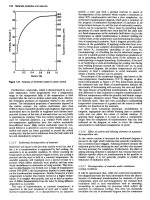
1.2.2 Exponential and hyperbolic relations

Exponential functions For a positive datum (`real')
number u, the exponential functions exp(u) and exp(�u)
are given by the summation to infinity of the series
3 4
expu@1 u u
2
=2! u =3!  u =4! @
with exp(u) increasing and exp(�u) decreasing at a rate
proportional to u.
If u 1, then
exp11 1  1=2 1=6  1=24 e  2:718 @
exp�11 �1  1=2 �1=6  1=24 �1=e  0:368 @
In the electrical technology of transients, u is most com-
monly a negative function of time t given by u �(t/T ).
It then has the graphical form shown in Figure 1.2 (left)
as a time dependent variable. With an initial value k, i.e.
y k exp(�t/T ), the rate of reduction with time is dy/dt @
�(k/T)exp(�t/T ). The initial rate at t 0is �k/T. If this
rate were maintained, y would reach zero at t T, defining
the time constant T. Actually, after time T the value of y is k
exp(� t/T ) k exp(�1) 0.368k. Each successive interval T
decreases y by the factor 0.368. At a time t 4.6T the value
of y is 0.01k, and at t 6.9T it is 0.001k.
Figure 1.1 Trigonometric relations
//integras/b&h/eer/Final_06-09-02/eerc001
1/8 Units, mathematics and physical quantities
Figure 1.3 Hyperbolic relations
If u is a quadrature (`imaginary') number jv, then
3 4
expjv1 jv �v

2
=2!  jv =3!  v =4! 
because j
2
�1, j
3
�j1, j
4
1, etc. Figure 1.2 (right)
shows the summation of the first five terms for exp(j1), i.e.
expj11 j1 �1=2 �j1=6  1=24
a complex or expression converging to a point P. The length
OP is unity and the angle of OP to the datum axis is, in fact,
1 rad. In general, exp(jv) is equivalent to a shift by v rad.
It follows that exp(jv) cos v  j sin v, and that
expjvexp�jv2 cos v expjv�exp�jvj2 sin v
For a complex number (u jv), then
expu jvexpuexpjvexpuv
Hyperbolic functions A point P on a rectangular hyper-
bola (x/a)
2
�@ (y/a)
2
1 defines the hyperbolic `sector' area
2
S
h

1
a ln[(x/a � (y/a)] shown shaded in Figure 1.3 (left). By

2
analogy with & 2S
c
/h
2
for the trigonometrical angle ,the
hyperbolic entity (not an angle in the ordinary sense) is
u 2S
h
/a
2
,where a is the major semi-axis. Then the hyperbolic
functions of u for point P are:
sinh u  y=a cosech u  a=y
cosh u  x=a sech u  a=x
tanh u  y=x coth u  x=y
Figure 1.2 Exponential relations
The principal relations yield the curves shown in the
diagram (right) for values of u between 0 and 3. For higher
values sinh u approaches cosh u, and tanh u becomes
asymptotic to 1. Inspection shows that cosh(�u) cosh u,
sinh(�u) �sinh u and cosh
2
u� sinh
2
u 1.
The hyperbolic functions can also be expressed in the
exponential form through the series
4 6
cosh u  1  u

2
=2!  u =4!  u =6! @
5 7
sinh u  u  u
3
=3!  u =5!  u =7! @
so that
cosh u 
1
expuexp�u@ sinh u 
1
expu�exp�u
2 2
cosh u sinh u  expu@ cosh u � sinh u  exp�u@
Other relations are:
sinh u sinh v  2 sinh
1
u  vcosh
1
u � v
2 2
cosh u cosh v  2 cosh
1
u  vcosh
1
u �v
2 2
cosh u �cosh v  2 sinh
1
u  vsinh

1
u �v
2 2
sinhu vsinh u cosh v  cosh u sinh v
coshu vcosh u cosh v  sinh u sinh v
tanhu vtanh u tanh v=1 tanh u tanh v@
//integras/b&h/eer/Final_06-09-02/eerc001
Mathematics 1/9
Table 1.8 Exponential and hyperbolic functions
u exp(u) exp(�u) sinh u cosh u tanh u
0.0 1.0 1.0 0.0 1.0 0.0
0.1 1.1052 0.9048 0.1092 1.0050 0.0997
0.2 1.2214 0.8187 0.2013 1.0201 0.1974
0.3 1.3499 0.7408 0.3045 1.0453 0.2913
0.4 1.4918 0.6703 0.4108 1.0811 0.3799
0.5 1.6487 0.6065 0.5211 1.1276 0.4621
0.6 1.8221 0.5488 0.6367 1.1855 0.5370
0.7 2.0138 0.4966 0.7586 1.2552 0.6044
0.8 2.2255 0.4493 0.8881 1.3374 0.6640
0.9 2.4596 0.4066 1.0265 1.4331 0.7163
1.0 2.7183 0.3679 1.1752 1.5431 0.7616
1.2 3.320 0.3012 1.5095 1.8107 0.8337
1.4 4.055 0.2466 1.9043 2.1509 0.8854
1.6 4.953 0.2019 2.376 2.577 0.9217
1.8 6.050 0.1653 2.942 3.107 0.9468
2.0 7.389 0.1353 3.627 3.762 0.9640
2.303 10.00 0.100 4.950 5.049 0.9802
2.5 12.18 0.0821 6.050 6.132 0.9866
2.75 15.64 0.0639 7.789 7.853 0.9919
3.0 20.09 0.0498 10.02 10.07 0.9951

3.5 33.12 0.0302 16.54 16.57 0.9982
4.0 54.60 0.0183 27.29 27.31 0.9993
4.5 90.02 0.0111 45.00 45.01 0.9998
4.605 100.0 0.0100 49.77 49.80 0.9999
5.0 148.4 0.0067 74.20 74.21 0.9999
5.5 244.7 0.0041 122.3 cosh u

tanh u

6.0 403.4 0.0025 201.7 sinh u 1.0
6.908 1000 0.0010 500 
1
2
exp(u)
sinhu jvsinh u cos vjcosh u sin v@
coshu jvcosh u  cos vjsinh u  sin v@

dsinh u=du @ cosh u sinh u du @ cosh u

dcosh u=du @ sinh u cosh u du @ sinh u
Exponential and hyperbolic functions of u between zero
and 6.908 are listed in Table 1.8. Many calculators can give
such values directly.
1.2.3 Bessel functions
Problems in a wide range of technology (e.g. in eddy
currents, frequency modulation, etc.) can be set in the form
of the Bessel equation
 
2
d

2
y 1 dy n

 @
1 �@
y @ 0
2
dx
2
x dx x
and its solutions are called Bessel functions of order n. For
n 0 the solution is
4
=2
2 6
=2
2
 4
2
J
0
x@1 �x
2
=2
2
x  4
2
�x  6
2
@

and for n 1, 2, 3 . . .
 
n 2 4
x x x
J
n
x@
1 �@ @ �@
2
n
n! 22n 2@ 2 42n 22n  4@
Table 1.9 givesvaluesof J
n
(x) for various values of n and x.
1.2.4 Series
Factorials In several of the following the factorial (n!) of
integral numbers appears. For n between 2 and 10 these are
2! @ 2 1/2! 0.5
3! @ 6 1/3! 0.1667
4! @ 24 1/4! 0.417 10
�1
5! @ 120 1/5! 0.833 10
�2
6! @ 720 1/6! 0.139 10
�2
7! @ 5 040 1/7! 0.198 10
�3
8! @ 40 320 1/8! 0.248 10
�4
9! @ 362 880 1/9! 0.276 10

�5
10! 3 628 800 1/10! 0.276 10
�6
Progression
Arithmetic a (a d) (a 2d) [a (n � 1)d]

1
n (sum of 1st and nth terms)
2
n
Geometric a ar ar
2
ar
n�1
a(1�r )/(1�r)
Trigonometric See Section 1.2.1.
Exponential and hyperbolic See Section 1.2.2.
Binomial
nn �1n �2@
1  x
n
@ 1  nx @
nn �1@
x
2
@
x
3
@
2! 3!

n!
�1
r
x
r
@
r!n �r!
n
a  x
n
@ a
n
1 x=a
//integras/b&h/eer/Final_06-09-02/eerc001
1/10 Units, mathematics and physical quantities
Binomial coefficients n!/[r!(n�r)!] are tabulated:
Term r @ 0 1 2 3 4 5 6 7 8 9 10
n 1 1 1
2 1 2 1
3 1 3 3 1
4 1 4 6 4 1
5 1 5 10 10 5 1
6 1 6 15 20 15 6 1
7 1 7 21 35 35 21 7 1
8 1 8 28 56 70 56 28 8 1
9 1 9 36 84 126 126 84 36 9 1
10 1 10 45 120 210 252 210 120 45 10 1
Power If there is a power series for a function f(h), it is
given by
ii@ iii

f hf 0hf
i
0h
2
=2!f

0h
3
=3!f

0@
h
r
=r!f
r
0@ Maclaurin@
ii
f x hf xhf
i
xh
2
=2!f x@
h
r
=r!f
r
x@ Taylor@
Permutation, combination
n
P

r
 nn � 1n � 2n �3 n �r  1n!=n �r!
n
C
r
1=r!nn�1n�2n�3 n�r 1  n!=r!n�r!
Bessel See Section 1.2.3.
Fourier See Section 1.2.5.
1.2.5 Fourier series
A univalued periodic wave form f() of period 2& is repre-
sented by a summation in general of sine and cosine waves
of fundamental period 2& and of integral harmonic orders n
(2, 3, 4, )as
f c
0
 a
1
cos &  a
2
cos 2& a
n
cos n& @
 b
1
sin &  b
2
sin 2& b
n
sin n& @
The mean value of f() over a full period 2& is

1

2&
c
0
@ f d&
2&
0
and the harmonic-component amplitudes a and b are
1

2&
1

2&
a
n
@ f cos n&  d;& b
n
@ f sin n&  d&
&
0
&
0
Table 1.10 gives for a number of typical wave forms the
harmonic series in square brackets, preceded by the mean
value c
0
where it is not zero.
1.2.6 Derivatives and integrals

Some basic forms are listed in Table 1.11. Entries in a given
column are the integrals of those in the column to its
left and the derivatives of those to its right. Constants of
integration are omitted.
1.2.7 Laplace transforms
Laplace transformation is a method of deriving the
response of a system to any stimulus. The system has a
basic equation of behaviour, and the stimulus is a pulse,
step, sine wave or other variable with time. Such a response
involves integration: the Laplace transform method
removes integration difficulties, as tables are available for
the direct solution of a great variety of problems. The pro
-
cess is analogous to evaluation (for example) of y 2.1
3.6
by transformation into a logarithmic form log
y 3.6 log(2.1), and a subsequent inverse transformation
back into arithmetic by use of a table of antilogarithms.
The Laplace transform (L.t.) of a time-varying function
f(t)is

1@
L f t  Fs@
exp�stf tdt
0
and the inverse transformation of F(s) to give f(t)is
L
�1
Fs  f tlim
1


j!&
expstFsds
2
�j!&
The process, illustrated by the response of a current i(t)in
an electrical network of impedance z to a voltage v(t)
applied at t 0, is to write down the transform equation
IsVs=Zs@
where I(s) is the L.t. of the current i(t), V(s) is the L.t. of the
voltage v(t), and Z(s) is the operational impedance. Z(s) is
obtained from the network resistance R, inductance L and
capacitance C by leaving R unchanged but replacing L by
Ls and C by 1/Cs. The process is equivalent to writing the
network impedance for a steady state frequency !& and then
replacing j!& by s. V(s) and Z(s) are polynomials in s: the
quotient V(s)/Z(s) is reduced algebraically to a form recog
-
nisable in the transform table. The resulting current/time
relation i(t) is read out: it contains the complete solution.
However, if at t 0 the network has initial energy (i.e. if
currents flow in inductors or charges are stored in capa-
citors), the equation becomes
IsVsUs=Zs@
where U(s) contains such terms as LI
0
and (1/s)V
0
for the
inductors or capacitors at t 0.

A number of useful transform pairs is listed in Table 1.12.
1.2.8 Binary numeration
A number N in decimal notation can be represented by an
ordered set of binary digits a
n
, a
n�2
, ., a
2
, a
1
, a
0
such that
N  2
n
a
n
 2
n�1
a
n�1
2a
1
 a
0
Decimal 1 2 3 4 5 6 7 8 9 10 100
Binary 1 10 11 100 101 110 111 1000 1001 1010 1100100
//integras/b&h/eer/Final_06-09-02/eerc001
Table 1.9 Bessel functions J

n
(x)
n J
n
(1) J
n
(2) J
n
(3) J
n
(4) J
n
(5) J
n
(6) J
n
(7) J
n
(8) J
n
(9) J
n
(10) J
n
(11) J
n
(12) J
n
(13) J
n

(14) J
n
(15)
0 0.7652 0.2239 �0.2601 �0.3971 �0.1776 0.1506 0.3001 0.1717 �0.0903 �0.2459 �0.1712 0.0477 0.2069 0.1711 �0.0142
1 0.4401 0.5767 0.3391 �0.0660 �0.3276 �0.2767 �0.0047 0.2346 0.2453 0.0435 �0.1768 �0.2234 �0.0703 0.1334 0.2051
2 0.1149 0.3528 0.4861 0.3641 0.0466 �0.2429 �0.3014 �0.1130 0.1448 0.2546 0.1390 �0.0849 �0.2177 �0.1520 0.0416
3 0.0196 0.1289 0.3091 0.4302 0.3648 0.1148 �0.1676 �0.2911 �0.1809 0.0584 0.2273 0.1951 0.0033 �0.1768 �0.1940
4 Ð 0.0340 0.1320 0.2811 0.3912 0.3567 0.1578 �0.1054 �0.2655 �0.2196 �0.0150 0.1825 0.2193 0.0762 �0.1192
5 Ð Ð 0.0430 0.1321 0.2611 0.3621 0.3479 0.1858 �0.0550 �0.2341 �0.2383 �0.0735 0.1316 0.2204 0.1305
6 Ð Ð 0.0114 0.0491 0.1310 0.2458 0.3392 0.3376 0.2043 �0.0145 �0.2016 �0.2437 �0.1180 0.0812 0.2061
7 Ð Ð Ð 0.0152 0.0534 0.1296 0.2336 0.3206 0.3275 0.2167 0.0184 �0.1703 �0.2406 �0.1508 0.0345
8 Ð Ð Ð Ð 0.0184 0.0565 0.1280 0.2235 0.3051 0.3179 0.2250 0.0451 �0.1410 � 0.2320 �0.1740
9 Ð Ð Ð Ð Ð 0.0212 0.0589 0.1263 0.2149 0.2919 0.3089 0.2304 0.0670 � 0.1143 �0.2200
10 Ð Ð Ð Ð Ð Ð 0.0235 0.0608 0.1247 0.2075 0.2804 0.3005 0.2338 0.0850 �0.0901
11 Ð Ð Ð Ð Ð Ð Ð 0.0256 0.0622 0.1231 0.2010 0.2704 0.2927 0.2357 0.0999
12 Ð Ð Ð Ð Ð Ð Ð Ð 0.0274 0.0634 0.1216 0.1953 0.2615 0.2855 0.2367
13 Ð Ð Ð Ð Ð Ð Ð Ð 0.0108 0.0290 0.0643 0.1201 0.1901 0.2536 0.2787
14 Ð Ð Ð Ð Ð Ð Ð Ð Ð 0.0119 0.0304 0.0650 0.1188 0.1855 0.2464
15 Ð Ð Ð Ð Ð Ð Ð Ð Ð Ð 0.0130 0.0316 0.0656 0.1174 0.1813
Values below 0.01 not tabulated.
//integras/b&h/eer/Final_06-09-02/eerc001
1/12 Units, mathematics and physical quantities
Table 1.10 Fourier series
Wave form Series
Sine: a sin & Cosine: a sin &
 
4 sin & sin 3& sin 5& sin 7&
Square: a
@ @ @ @
& 1 3 5 7

 
2
p
3 sin & sin 5& sin 7& sin 11& sin 13& sin 17&
Rectangular block: a
� �   �@ �@
& 1 5 7 11 13 17

4 sin & sin 3& sin 5& sin 7& sin 9& sin 11&
Rectangular block: a
�   � @
& 2  1 3 2  5 2  7 9 2 11

sin 13& sin 15& sin 17&
@
�@ @ @
2 13 15 2 17
 
3 sin & sin 5& sin 7& sin 11& sin 13& sin 17&
Stepped rectangle: a
  @ @ @ @
& 1 5 7 11 13 17

3
p
3 sin & sin 5& sin 7& sin 11& sin 13&
Asymmetric rectangle: a
� � @ @ �@
2& 1 5 7 11 13
cos 2& cos 4& cos 8& cos 10&

� �  @ �@
2 4 8 10
 
8 sin & sin 3& sin 5& sin 7& sin 9& sin 11&
Triangle: a
�  �  �@ @

2
1 9 25 49 81 121
 
3 sin & sin 2& sin 3& sin 4& sin 5&
Sawtooth: a
�@ @ �@ @ �@
& 1 2 3 4 5
 
4 sin & sin & sin 3&  sin 3& sin 5&  sin 5&
Trapeze: a
@ @ @
& 1 9 25
 
6
p
3 sin & sin 5& sin 7& sin 11&
a
�@ @ �@ @ for =/3

2
1 25 49 121
 
9 sin & sin 5& sin 7& sin 11& sin 13&

Trapeze-triangle: a
 � @ �@ @

2
1 25 49 121 169
cont'd
//integras/b&h/eer/Final_06-09-02/eerc001
Mathematics 1/13
Table 1.10 (continued )
Wave form Series
 
1 2 & sin & cos 2& cos 4& cos 6&
Rectified sine (half-wave): a
 a �@ �@ �@ �@
 & 4 1 3 3  5 5 7
 
2 4 cos 2& cos 4& cos 6& cos 8&
Rectified sine (full-wave): a
� a @ @ @ @
 & 1  3 3 5 5 7 7 9
 
m & 2m & cos m& cos 2m& cos 3m&
Rectified sine (m-phase): a
sin  a sin
�@ @ �@
& m & m m
2
� 1 4
m
2

� 1 9
m
2
� 1
 
& 2 sin &  cos & sin 2&  cos 2& sin 3&  cos 3&
Rectangular pulse train: a
 a @ @ @
 & 1 2 3
 
& 2& cos & cos 2& cos 3&
a
 a @ @ @ for & @ &
 & 1 2 3

1 1 1
& 4
sin
2

2
@ sin
2
2@ @ sin
2
3@ 
2
Triangular pulse train: a
a
cos@

2
cos2@ cos3@
2& &
1 4 9
 &
a
a coscos2 cos 3 @ for & &
2 &
where the as have the values either 1 or 0. Thus, if N 19,
19 16 2 1 (2
4
)1 (2
3
)0 (2
2
)0 (2
1
)1 (2
0
)1 10011
in binary notation. The rules of addition and multiplication
are
0 0 0, 0 1 1, 1 1 10; 00 0, 01 0, 11 1
1.2.9 Power ratio
In communication networks the powers P
1
and P
2
at
two specified points may differ widely as the result of ampli-

fication or attenuation. The power ratio P
1
/P
2
is more
convenient in logarithmic terms.
Neper [Np] This is the natural logarithm of a voltage or
current ratio, given by
a @ lnV
1
=V
2
@ or a @ lnI
1
=I
2
 N
p
If the voltages are applied to, or the currents flow in,
identical impedances, then the power ratio is
a @ lnV
1
=V
2

2
@ 2lnV
1
=V
2

@
and similarly for current.
Decibel [dB] The power gain is given by the common
logarithm lg(P
1
/P
2
) in bel [B], or most commonly by
A 10 log(P
1
/P
2
) decibel [dB]. With again the proviso
that the powers are developed in identical impedances, the
power gain is
A @ 10 logP
1
=P
2
@10 logV
1
=V
2

2
@ 20 logV
1
=V
2
 dB

Table 1.13 gives the power ratio corresponding to a gain
A (in dB) and the related identical-impedance voltage (or
current) ratios. Approximately, 3 dB corresponds to a
power ratio of 2, and 6 dB to a power ratio of 4. The decibel
equivalent of 1 Np is 8.69 dB.
1.2.10 Matrices and vectors
1.2.10.1 Definitions
If a
11
, a
12
, a
13
, a
14
is a set of elements, then the rectangu-
lar array


a
14
a
1n
a
11
a
12
a
13


a
24
a
2n

a
21
a
22
a
23


A @


a
m1
a
m2
a
m3
a
m4
a
mn
arranged in m rows and n columns is called an (m n)
matrix.If m n then A is n-square.