InTech-Design_of_a_parallel_robotic_manipulator_using_evolutionary_computing
Bạn đang xem bản rút gọn của tài liệu. Xem và tải ngay bản đầy đủ của tài liệu tại đây (2.71 MB, 13 trang )
International Journal of Advanced Robotic Systems
Design of a Parallel Robotic Manipulator
using Evolutionary Computing
Regular Paper
António M. Lopes
1,*
, E.J. Solteiro Pires
2
and Manuel R. Barbosa
1
1 IDMEC – Pólo FEUP, Faculdade de Engenharia, Universidade do Porto, Portugal
2 Centro de Investigação e de Tecnologias Agro-Ambientais e Biológicas,
Escola de Ciências e Tecnologia da Universidade de Trás-os-Montes e Alto Douro, Portugal
* Corresponding author E-mail:
Received 27 Oct 2011; Accepted 14 Mar 2012
DOI: 10.5772/50922
© 2012 Lopes et al.; licensee InTech. This is an open access article distributed under the terms of the Creative
Commons Attribution License ( which permits unrestricted use,
distribution, and reproduction in any medium, provided the original work is properly cited.
Abstract In this paper the kinematic design of a 6‐dof
parallel robotic manipulator is analysed. Firstly, the
condition number of the inverse kinematic jacobian is
considered as the objective function, measuring the
manipulator’s dexterity and a genetic algorithm is used to
solve the optimization problem. In a second approach, a
neural network model of the analytical objective function
is developed and subsequently used as the objective
function in the genetic algorithm optimization search
process. It is shown that the neuro‐genetic algorithm can
find close to optimal solutions for maximum dexterity,
significantly reducing the computational burden. The
sensitivity of the condition number in the robot’s
workspace is analysed and used to guide the designer in
choosing the best structural configuration. Finally, a
global optimization problem is also addressed.
Keywords Robotics, Parallel Manipulator, Optimization,
Genetic Algorithm, Neural Network
1. Introduction
The advantages of manipulators based on parallel design
architectures, compared to the serial‐based ones, are well
recognized and justified by the increasing number of
applications which, nowadays, try to explore their
inherent low positioning errors and
high dynamic
performance [1‐2]. Among these applications, references
can be made to robot manipulators and robotic end‐
effectors, high speed machine‐tools and robotic high‐
precision tasks, flight simulators and haptic devices [3].
In spite of the inherent general characteristics, the choice
of a specific structural configuration and its dimensioning
remains a complex problem, as it involves the
specification of several design parameters and the
consideration of different performance criteria [30].
Optimizing the design to suit a foreseen application
remains, therefore, an active area of research.
Optimization based on the manipulator workspace [4‐6] is
the area upon which most of the research concentrates as it
represents one of the main disadvantages, when compared
to serial manipulators. In an alternative way, which seeks
to explore the parallel manipulator’s main advantages,
other authors choose to optimize the structural stiffness
[7‐9]. Several works may also be referred to where the
optimization criteria are related with the manipulability, or
1
António M. Lopes, E.J. Solteiro Pires and Manuel R. Barbosa:
Design of a Parallel Robotic Manipulator using Evolutionary Computing
www.intechopen.com
ARTICLE
www.intechopen.com
Int J Adv Robotic Sy, 2012, Vol. 9, 26:2012
dexterity, of the manipulator [10‐14]. Finally, objective
functions based on the manipulator natural frequencies
have also been considered [31‐32].
Optimization can be a difficult and time consuming task,
because of the great number of optimization parameters
and the complexity of the objective functions involved.
However, optimization procedures based on evolutionary
approaches have been proved as an effective solution
[15‐17, 29].
In this paper the kinematic design of a 6‐dof parallel
robotic manipulator for maximum dexterity is analysed.
The condition number of the inverse kinematic jacobian is
used as a measure of dexterity and a Genetic Algorithm
(GA) is used to solve the optimization problem. The
highly nonlinear nature of the problems involved and
the, normally, time consuming optimization algorithms
that are used can be naturally approached by artificial
Neural Networks (NNs) techniques. In order to explore
the advantages of NNs and GAs, a neuro‐genetic
formulation is developed and tested. In our work we
quantify the error of the NN’s approximation through
testing and validating data sets, and we present a direct
comparison of the optima obtained using as the fitness
function, either the NN’s approximation or the analytical
function. This has not been directly
addressed in existing
research (e.g., [15]).
It is shown that the neuro‐genetic algorithm can find
close to optimal solutions for maximum dexterity,
significantly reducing the computational burden.
Local optimization criteria are especially useful when
applied to manipulators with small workspaces, or
designed to operate over a small subset of their
workspaces. Therefore, a global optimization problem is
also addressed and solved.
The paper is organized as follows. Section 2 presents the
manipulator architecture and kinematics. In section 3 the
optimization problem is formulated and solved using a
GA. Section 4 presents a neuro‐genetic formulation. In
section 5 sensitivity analysis is carried out. In section 6 the
global optimization problem is considered and, finally,
conclusions are drawn in section 7.
2. Manipulator Architecture and Kinematics
The mechanical architecture of the parallel robot
comprises a fixed (base) planar platform and a moving
(payload) planar platform, linked together by six
independent, identical, open kinematic chains (Figure 1).
Each chain comprises two links: the first link (linear
actuator) is always normal to the base and has a variable
length, l
i
, with one of its ends fixed to the base and the
other one attached, by a universal joint, to the second
link; the second link (arm) has a fixed length, L, and is
attached to the payload platform by a spherical joint.
Points B
i
and P
i
are the connecting points to the base and
payload platforms. They are located at the vertices of two
semi‐regular hexagons, inscribed in circumferences of
radius r
B
and r
P
, that are coplanar with the base and
payload platforms (Figure 2).
Figure 1. Schematic representation of the parallel manipulator
architecture.
For kinematic modelling purposes, a right‐handed
reference frame {B} is attached to the base. Its origin is
located at point B, the centroid of the base. Axis x
B
is
normal to the line connecting points B
1
and B
6
and axis z
B
is
normal to the base, pointing towards the payload platform.
The angles between points B
1
and B
3,
and points B
3
and B
5
are set to 120°. The separation angles between points B
1
and
B
6
, B
2
and B
3
, and B
4
and B
5
are denoted by 2
B
(Figure 2).
In a similar way, a right‐handed frame {P} is assigned to
the payload platform. Its origin is located
at point P, the
centroid of the payload platform. Axis x
P
is normal to the
line connecting points P
1
and P
6,
and axis z
P
is normal to
the payload platform, pointing in a direction opposite to
the base. The angles between points P
1
and P
3,
and points
P
3
and P
5
are set to 120°. The separation angles between
points P
1
and P
2
, P
3
and P
4
, and P
5
and P
6
are denoted by
2
P
(Figure 2) [33].
Taking into account the definitions given above, the
generalized position of frame {P} relative to frame {B}
may be represented by the vector:
TT
E
oP
BT
B
posP
B
T
PPPPPP
EB
P
B
zyx
][
|
xx
x
(1)
where
T
PPP
B
posP
B
zyxx
is the position of the
origin of frame {P} relative to frame {B}, and
2
Int J Adv Robotic Sy, 2012, Vol. 9, 26:2012 www.intechopen.com
T
PPP
E
oP
B
x
defines an Euler’s angle system
representing the orientation of frame {P} relative to {B}.
Vector
T
iz
P
iy
P
ix
P
i
P
pppp represents the position of
point P
i
with respect to frame {P} and vector
T
iziyixi
bbbb
represents the position of point B
i
with
respect to frame {B}.
Figure 2. Position of the connecting points on the base and
payload platform.
2.1 Inverse Position Kinematics
The inverse position kinematic model is used to compute
the joints positions for a given Cartesian position and
orientation. The presented model follows the one
proposed in [18].
Taking into account a single kinematic chain, i, vector
p
p
i
may be written in the base frame using the following
transformation:
iz
P
iy
P
ix
P
iz
P
iy
P
ix
P
iz
P
iy
P
ix
P
i
P
P
B
B
i
P
prprpr
prprpr
prprpr
333231
232221
131211
pRp (2)
where
B
R
P
is a matrix representing the orientation of the
payload platform frame with reference to the base frame,
that may be computed from the Euler’s angles (
P
,
P
,
P
).
Subtracting vectors
B
posP
B
x and b
i
, then vector
T
iziyixi
ssss
is obtained. If s
i
and
B
i
P
p are added, the
vector
T
iziyixi
eeee
is obtained, that is:
iz
P
iy
P
ix
P
iz
P
iy
P
ix
P
iz
P
iy
P
ix
P
izP
iyP
ixP
B
i
P
i
B
i
P
i
B
posP
B
i
prprpr
prprpr
prprpr
bz
by
bx
333231
232221
131211
pspbxe
(3)
Vector a
i
, aligned with the fixed length arm, is given by
ai = ei di. Where d
i
is a vector parallel to z
B
, and length l
i
(Figure 3).
Figure 3. Schematic representation of a kinematic chain.
Knowing that the 2‐norm of a
i
is equal to the arm length,
L, it follows that:
L
iii
22
dea
(4)
Lleee
iiziyix
2
22
(5)
Solving for l
i
results in
222
iyixizi
eeLel
(6)
that is, there are two possible solutions for l
i
. The
solutions corresponding to the manipulator having the
universal joints below the payload platform spherical
joints are always considered:
222
iyixizi
eeLel
(7)
2.2 Inverse Velocity Kinematics
The inverse velocity kinematics can be represented by the
inverse kinematic jacobian, relating the joints velocities to
the manipulator Cartesian‐space velocities (linear and
angular) [18]:
B
P
B
C
xJl
(8)
Payload
platform
Base
3
António M. Lopes, E.J. Solteiro Pires and Manuel R. Barbosa:
Design of a Parallel Robotic Manipulator using Evolutionary Computing
www.intechopen.com
Vector
T
lll
621
l represents the joints velocities,
and vector
T
T
B
P
BT
B
posP
B
B
P
B
ωxx
represents the
Cartesian‐space velocities.
The velocity of point P
i
is dependent upon the linear and
angular velocities of the payload platform. If
B
P
B
i
v
denotes that velocity with respect to the base frame (and
written in that same frame), then:
B
i
P
B
P
B
B
posP
B
i
B
P
B
i
pωxpv
(9)
where
B
P
B
B
posP
B
vx
and
B
P
B
ω represent the linear and
angular velocities of the payload platform frame with
respect to, and written in, the base frame.
Squaring both sides of equation (4), the following relation
is obtained:
i
T
ii
T
ii
T
ii
T
i
edeeddaa 2 (10)
Differentiating equation (10), the following expression
results:
0
i
T
Bii
T
Bii
T
iii
llll ezezee
(11)
where z
B
= 0 0 1
T
denotes the direction of displacement
of the linear actuators.
From equation (11), and taking into account that
ii
pe
,
an expression for the linear actuators velocity,
i
l
, is
obtained:
B
P
B
ii
T
B
T
Bii
B
i
P
B
posP
B
ii
T
B
T
Bii
i
l
l
l
l
l ω
ez
zep
x
ez
ze
(12)
Following this result, the inverse kinematic jacobian may
be written (with respect to the base frame) as:
66
66
6
66
66
11
11
1
11
11
l
l
l
l
l
l
l
l
T
B
T
B
B
P
T
B
T
B
T
B
T
B
B
P
T
B
T
B
C
ez
zep
ez
ze
ez
zep
ez
ze
J (13)
3. Optimization
3.1 Objective Function
Several performance indexes can be formulated based on
the manipulator inverse kinematic jacobian [34].
In this work we consider the condition number of the
inverse kinematic jacobian matrix, J
C
. The condition
number is configuration‐dependent and may take values
between unity (isotropic configuration) and infinity
(singular configuration). The minimization of the
condition number leads not only to the maximization of
the manipulator dexterity, but also to the minimization of
the error propagation due to actuators, feedback
transducers and, when the J
C
matrix is inverted,
numerically induced noise [19].
For example, Salisbury and Craig [20] used the condition
number of the jacobian matrix to optimize the finger
dimensions of an articulated hand. At the same time they
introduced the concept of isotropic configuration, that is,
a configuration (mechanical architecture and pose)
presenting a condition number equal to one. In an
isotropic configuration a
manipulator will require equal
joint effort to move or produce forces and/or torques in
each direction.
Mathematically, the condition number is given by
Cmin
Cmax
J
J
(14)
where
Cmax
J
and
Cmin
J
represent the maximum and
minimum singular values of the matrix J
C
.
For a 6‐dof parallel manipulator, in order to obtain a
dimensionally homogeneous jacobian matrix, some kind
of normalization procedure has to be used. In this case we
use the manipulator payload platform radius, r
P
, as a
characteristic length. In this way, the same ‘cost’ will be
associated to translational and rotational movements of
the payload platform. Using r
P
as the length unit, the
inverse kinematic jacobian results depend upon ten
variables, four of them being manipulator kinematic
parameters: the position and orientation of the payload
platform; the base radius (r
B
); the separation angles on the
payload platform (
P
); the separation angles on the base
(
B
); and the arm length (L).
The optimization is done for the manipulator lying in one
single configuration (position and orientation); in
particular in the centre of the workspace, [0 0 2 0 0 0]
T
(units in r
P
and degrees, respectively). Thus, for this pose,
the jacobian matrix is a function of the four kinematic
parameters.
3.2 Genetic Algorithm‐Based Approach
A genetic approach is used to optimize the objective
function. The proposed
GA uses a real value chromosome
given by the four robot kinematic parameters, p = [r
B
P
B
L]
T
. At the beginning of the algorithm, the solutions are
randomly initialized in the range 1.0 r
B
2.5, 0°
P
,
B
25° and 2.0 L 3.5. Next, during the generations, a
tournament‐2 selection is used to determine the parents
4
Int J Adv Robotic Sy, 2012, Vol. 9, 26:2012 www.intechopen.com
of the new offspring [22]. After selection, the simulated
binary crossover and mutation operators with p
c
= 0.6 and
p
m
= 0.05 probabilities, respectively, are called [23]. At the
end of each generation, a
)(
strategy is used to
select the solutions which survive for the next iteration.
Thus, the best solutions among parents and offspring are
always chosen. At this stage, the space is divided into
hyper‐planes separated by the distance
and all solutions
that fall into two consecutive hyper‐planes are considered
as having the same preference, even if their fitness values
are different [24]. Two consecutive hyper‐planes define a
rank. In order to sort the solutions in a rank, the maximum
selection is used [25‐26]. The
value is initialized with 20
and is decreased during the evolution, until it reaches the
value 0.003. The
is decreased by 90% every time the best
200 solutions belong to the first rank and the value has not
changed during the last 100 generations.
The solutions are classified according to the fitness
function given by equation (14), in case the solution is
admissible, otherwise a large value (1×10²⁰) is assigned.
The global results (Figures 4 and 5) show that there are
multiple sets of kinematic parameters that are optimal.
Moreover, the algorithm draws a representative solution
set of the optimal parameters front. It can be seen, in
Figure 5. that the final population set belongs to the best
rank (
)min()max( fitnessfitness
).
4. Neuro‐Genetic Algorithm‐Based Approach
Artificial Neural Networks (NNs) can be considered a
problem solving tool with specific characteristics that can
be of interest for the development of alternative solutions,
to a vast range of problems. In this work we are mainly
interested in exploring the well‐known capability of NNs
to approximate complicated nonlinear functions [27‐28],
when applied to the objective functions associated with
the optimal design of parallel manipulators.
The particular structure of NNs solutions, which is based
on the use of a high number of simple processing
elements and the respective interconnections, creates a
mapping function tool with a high number of adjustable
parameters. The process of adjusting these parameters
requires the availability of data represented by instances
of the problem. Although the design phase can be time
consuming and therefore, normally performed in an off‐
line mode, a
trained NN consists of a well‐defined and
deterministic set of operations which provide an instant
solution to a specific instance of the problem, provided it
has learned and generalized well.
Our objective was therefore, at this stage, to evaluate the
performance of an NN developed to map the condition
number function of the inverse jacobian, κ, of equation (14).
Figure 4. Simulation results: optimal sets of kinematic
parameters. The marked points are used in in the sensitivity
analysis (section 5). The observed small differences in the
numerical values are due to the finite resolution of the mesh.
5
António M. Lopes, E.J. Solteiro Pires and Manuel R. Barbosa:
Design of a Parallel Robotic Manipulator using Evolutionary Computing
www.intechopen.com
Figure 5. Simulation results: fitness function values for 200 sets
of optimal solutions.
4.1 Development of an Artificial Neural Network Mapping of
the Objective Function
The process of designing an NN solution to a specific
problem is mainly guided by trial and experimentation,
due to the lack of explicit and proven methods that can be
used to choose and set the various parameters involved
in the NN design process.
Among the different structures and types of NN
available, the experiments were done using classical
multilayer feedforward architecture. However, instead of
using the standard backpropagation learning algorithm,
training was performed using the Levenberg‐Marquardt
(LM) algorithm, which represents a faster alternative and
also benefits from an efficient implementation in Matlab
®
software.
The representation of the problem in this multilayer NN
structure was to provide at the input layer the four
kinematic parameters (r
B
,
P
,
B
, L) and to produce the
condition number of the inverse jacobian (κ) at the output
layer (Figure 6). The number of intermediate layers, i.e.,
hidden layers, and the respective number of hidden
elements were established based on multiple experiments
with various combinations. From these experiments,
networks with one
hidden layer and three different
numbers of hidden elements (25, 50, and 100) were
selected.
Figure 6. Feedforward NN elements (4 Inputs, 1 Hidden layer,
1 Output).
The data used to develop the networks was obtained by
generating random values for each of the four arguments
and eliminating the impossible combinations (i.e.,
negative κ values). The cases generated were split into
training (70%), validating (15%) and testing (15%) data
sets. As can be observed in Figure 7, the three sets have
similar distributions. Furthermore, the cases with lowest
κ values (i.e., below 2.0) are very few (five in total) and
most cases are also well below the maximum values
obtained. The minimum and maximum values for these
sets are: TRA(1.4656; 12.0140), VAL(1.4170; 10.7360) e
TES(1.4545; 10.2760).
The training and testing steps performed in each
experiment followed common procedures, such as
normalizing the data cases used, starting the learning
process from different random initial states and
observing performance along the training iterations. The
performance measure used was the mean square error
function (mse), calculated for each of the three data sets,
as can be observed in Figure 8. The learning process was
controlled based on the behaviour of the mse function, i.e.,
the number of successive increases, on the validation set.
Figure 7. Histogram representation of the κ value’s distribution
for the three data sets: training (TRA), 6999 cases, validating
(VAL), 1500 cases and testing (TES), 1500 cases.
Figure 8. Performance measure (mse) evolution during the
training iterations (epochs): training (TRA), validating (VAL)
and testing (TES) data sets.
0 20 40 60 80 100 120 140 160 180 200
1.414
1.4145
1.415
1.4155
1.416
1.4165
1.417
1.4175
1.418
Fitness
Iteration
0,1
1
10
100
1000
1
2
3
4
5
6
7
8
9
10
11
12
13
TRA
VAL
TES
0 200 400 600 800 1000 1200 1400 1600
10
-8
10
-6
10
-4
10
-2
10
0
10
2
Number of Epochs
MSE-Mean Square Error [Log Scale]
TRA VAL TES
6
Int J Adv Robotic Sy, 2012, Vol. 9, 26:2012 www.intechopen.com
Subsequent to the learning process, the performance of
the trained network was analysed, after reverting
normalization in the data sets, through the maximum and
minimum error values and the root mean square error
(rmse) (Table 1). Considering the range of values of the
objective function included in the data sets [1.4170,
12.0140], the results obtained with mapping the objective
function using NNs show that a good approximation is
possible in average terms (i.e.,
mse
0.01). Analysing
the maximum and minimum error values, they can be
larger by more than one order of magnitude (i.e., 0.50,
Table 1), but 98% of the absolute values of the errors in
the data used fall below 0.01.
Having developed an NN approximation of the condition
number of the inverse jacobian (κ), the objective was to
evaluate whether the NN approximation could be used, as
the fitness function, in a search for minimum values
through GAs. In this way it will open up an opportunity to
use NNs in the optimal design of parallel manipulators.
Table 1. Performance of a neural network with 50 hidden
elements, relative to desired output (i.e., Target‐NN output),
after reversing normalization: square root of mean square error (
mse
), maximum (Max) and minimum (Min) error values.
The experiments performed in the minimization search
use various NN approximations and also the analytical
function. In each search, the 200 best cases found were
considered for comparison. Figure 9 illustrates the results
obtained using NNs with a different number of hidden
elements (25, 50, and 100) and with the analytical
function. It can be observed that in general the GA
process using NNs converged to minimum values of the
approximated function. However, these values were well
above the minimum values, i.e., [1.41 to 1.42], obtained
when using the analytical function. Furthermore, the
smaller the network sizes, in general, the approximated
values are reduced to a minimum.
The higher minimum values of the NNs’ approximations
can be explained considering the distribution of the data
sets used to develop the NNs (Figure 7). Only five cases
(two in the training set, two in the validating set and one
in the testing set) were cases with a k value below 2.0.
This also supports the common belief that NNs are better
interpolators than as extrapolating.
Comparing the series of minimum values obtained with the
different NNs, the NNs with a
lower number of elements in
the hidden layer converged to lower values in the
minimization process. This also seems to agree with the
belief that smaller networks will tend to generalize better
than larger networks. To complement this analysis, a
comparison of the approximation values provided by each
network with the real values can be observed in Figure 10
(50 hidden elements network) and Figure 11 (25 hidden
elements network). It can be observed that the smaller size
NN, provides lower approximated k values (Figure 9), which
also represent lower real values (Figure 11). However, when
compared to a larger size network, in Figures 9 and 11, they
are more dispersed. In addition, they include more cases
where the NN’s approximation is below the real value.
From these experiments it can be said that an
approximation to complex functions by an NN can be used
in the process of finding optimum solutions for the design
of parallel manipulators. In spite of their inherent
limitations to extrapolate well to the minimum values of a
function, they converge to close to minimum values, which
in a multi‐criteria optimization problem may be less
significant. Furthermore, the use of the GA‐NN based
approach was able to reduce the search time by 30% to
50%, compared to the use of a GA analytical function. The
time to develop the NN is not included, but in a case where
the analytical function is also not available, such for
example, on a multi‐criteria optimization case, this as well,
adds favourably to the advantages of NN‐based solutions.
Figure 9. Values of the objective function (κ) for each of the 200
considered best cases: GA‐Analytical Func., GA‐NN25 Hid. El.,
GA‐NN50 Hid. El., GA‐NN100 Hid. El.
Figure 10. Values of the objective function (κ) for each of the 200
considered best cases using 50 Hidden Ele. NN: values of the
analytical function and values of the NN approximation.
20 40 60 80 100 120 140 160 180 200
1.41
1.42
1.43
1.44
1.45
1.46
1.47
1.48
1.49
1.5
1.51
Best Cases
Obje ctive Functio n (k )
GA-Anal.F. GA-NN25 GA-NN50 GA-NN100
20 40 60 80 100 120 140 160 180 200
1,41
1,42
1,43
1,44
1,45
1,46
1,47
1,48
1,49
1,5
1,51
Best 200 Cases
Objective Function (k)
Analytical Func (k) NN-50Hid.El.
NN ‐ 50 Hid. Elements
mse
Max Min
Training 0.0034 0.0543 ‐0.0490
Validating 0.0135 0.0742 ‐0.5016
Testing 0.0093 0.3304 ‐0.0726
7
António M. Lopes, E.J. Solteiro Pires and Manuel R. Barbosa:
Design of a Parallel Robotic Manipulator using Evolutionary Computing
www.intechopen.com
Figure 11. Values of the objective function (κ) for each of the 200
considered best cases using the 25 Hidden Ele. NN: values of the
analytical function and values of the NN approximation.
5. Sensitivity Analysis
As seen in the previous sections, the optimization
algorithm draws a representative solution set of the front
of optimal parameters. As the robot designer has to
choose one optimal solution among a large set of
candidates, additional information must be provided to
support her/his job.
(a) (b)
Figure 12. Schematic representation of the parallel manipulator
for two optimal solutions (a) configuration 1; (b) configuration 2.
In this section a sensitivity analysis is presented, showing
how the analytical objective function,
, evolves inside a
given workspace. Two representative, and almost
opposite, optimal solutions are considered. Configuration
1 (Figure12a) corresponding to the set of parameters [r
B
P
B
L]
T
= [2.0113r
P
0° 0° 2.4643r
P
]
T
, which means a 3‐3 type
architecture (triangular base and payload platforms) with
a large L and configuration 2, described by the kinematic
parameters [1.7321r
P
0° 5.2635° 2.0000r
P
]
T
, corresponding
to a 6‐3 type architecture
(hexagonal base and triangular
payload platform) with a shorter L (Figure 12 b). Usually,
larger values of L are desirable in order to have larger
workspaces.
Figures 13 to 16 show the variation of
in a given
manipulator workspace. The workspace is described by a
mesh of points on the surface of a sphere with radius 0.3
r
P
. The centre of the mobile platform is then positioned in
all points of the mesh and rotated by an angle between
‐30° and 30° in any direction. At each point of the
discretized workspace the condition number,
, was
evaluated. As can be seen in the figures 13 to 16,
, is
minimum at the centre of the workspace, getting higher
as the distance to the centre increases. Moreover, it can be
noticed that configuration 2 is more sensitive to the
distance than configuration 1, because
increases faster.
(a)
(b)
Figure 13. Variation of
with respect to x and y (a) for
configuration 1; (b) for configuration 2.
On the other hand, for the workspace mentioned above,
the maximum displacement of the actuators and the
extreme values of
and singular values were analysed.
Table 2 shows the main results.
Configuration #1 Configuration #2
Value Value
l
i
2.0123 r
P
2.1648 r
P
min
1.4940 1.5092
max
2.9908 6.4506
min
1.6888 1.6815
max
2.4525 2.4541
Table 2. Maximum actuators displacement and extreme values
of
and singular values.
Figures 18 and 19 represent the manipulator poses
corresponding to the parameters shown in Table 2, for the
two considered configurations.
20 40 60 80 100 120 140 160 180 200
1.41
1.42
1.43
1.44
1.45
1.46
1.47
1.48
1.49
1.5
1.51
1.52
Best 200 Cases
Objective Function (k)
Analytical Func (k) NN-25Hid.El.
8
Int J Adv Robotic Sy, 2012, Vol. 9, 26:2012 www.intechopen.com
(a)
(b)
Figure 14. Variation of
with respect to
and
(a) for
configuration 1; (b) for configuration 2.
According to the sensitivity analysis, it might be
concluded that configuration 1 will correspond to the best
performance.
A triangular payload platform results in double spherical
joints connecting the kinematic chains to that platform.
As the mechanical solution for this is well known, the
main disadvantage is the propensity to increase kinematic
chain interference, because the physical dimensions of the
links are usually bigger.
A triangular base platform results in three pairs of
coincident actuators, leading to an even more
complicated mechanical design. Therefore, a trade‐off
must be taken into account between better performance
and harder mechanical design.
(a)
(b)
Figure 15. Variation of
with respect to
and
(a) for
configuration 1; (b) for configuration 2.
Similar results were obtained when the sensitivity
analysis was carried out using the NN approximated
objective function. Figure 17 illustrates one representative
case of an NN solution (green surface) and a comparable
analytical solution (red surface) in terms of dexterous
workspace; a very similar behaviour can be observed. The
NN solution is only clearly
over the analytical solution
farther away from the centre of the workspace. This goes
in line with the GA‐NN solutions, in general providing
slightly worst solutions, but faster computational times.
9
António M. Lopes, E.J. Solteiro Pires and Manuel R. Barbosa:
Design of a Parallel Robotic Manipulator using Evolutionary Computing
www.intechopen.com
(a)
(b)
Figure 16. Variation of
with respect to
and
(a) for
configuration 1; (b) for configuration 2.
Figure 17. Variation of
with respect to x and y, for
configuration 1. The red surface is the result obtained using the
analytical objective function; the green one corresponds to the
function given by the NN.
(a) (b)
(c) (d)
Figure 18. Manipulator poses corresponding extreme values of
and singular values for configuration 1 (a)
min
; (b)
max
; (c)
min
;
(d)
max.
(a) (b)
(c) (d)
Figure 19. Manipulator poses corresponding to extreme values of
and singular values for configuration 2 (a)
min
; (b)
max
; (c)
min
;
(d)
max.
6. Global Optimization
In this section the previous approach is generalized and
used in a global optimization problem. The objective
function is the global index given by equation (15).
10
Int J Adv Robotic Sy, 2012, Vol. 9, 26:2012 www.intechopen.com
W
W
dW
dW
1
(15)
where the reciprocal of the condition number is evaluated
in the manipulator workspace, W. The reciprocal of the
condition number is used because it is numerically better
behaved. Equation (15) is approximated by
n
i
i
n
1
11
(16)
where the value of
is calculated after discretization of
the manipulator workspace and computation of 1/
at
each of the n points of the resulting mesh.
For simulation, to reduce the computational load, we
consider the particular case of a manipulator having a
triangular payload platform,
P
= 0. The workspace is the
hyper‐volume defined by ‐0.4
x
P
, y
P
, z
P
0.4 for translations
(units in r
P
), and ‐25°
P
,
P
,
P
25° for rotations. The
allowed variation of the manipulator parameters is 1.0
r
B
2.5 r
P
, 0°
B
25° and 3.0
L
4.5 r
P
.
Figure 20 illustrates the evolution of the global index
versus the manipulator parameters. It can be seen, for a
given solution of the optimal set, [r
B
B
L] = [2.5 0 3.6], that
the global index degrades considerably as a consequence
of optimal parameters detuning.
7. Conclusions
In this paper the kinematic design of a 6‐dof parallel
robotic manipulator for maximum dexterity was
analysed. First, a
GA was utilized to solve the
optimization problem. Afterwards, a neuro‐genetic
formulation was developed and tested. The GA
converged to optimal solutions characterized by multiple
sets of optimal kinematic parameters. Moreover, the GA
provides a representative solution set of the parameters
front. NNs were used to map nonlinear objective
functions associated with the design of parallel
manipulators. The performance obtained showed they
can be used as the fitness function in a GA minimization
process, reducing the computational time. Since the
optimization algorithm draws several optimal solutions, a
sensitivity analysis was performed in order to guide the
robot designer to select the best structural configuration.
Although the final solutions have all the same objective
value,
, the analysis reveals that some architectures
might be preferred. The approach can be easy generalized
and used in a global optimization problem.
(a)
(b)
(c)
Figure 20. Global index vs. (a) (L, r
B
),
B
= 0; (b) (L,
B
), r
B
= 2.5;
(c) (r
B
,
B
), L = 3.6.
8. References
[1] D. Chablat, P. Wenger, F. Majou, J.‐P. Merlet, “An
Interval Analysis Based Study for the Design and the
Comparison of Three‐
Degrees‐of‐Freedom Parallel
Kinematic Machines,” The International Journal of
Robotics Research, vol. 23, pp. 615‐624, 2004.
[2] M. Z. Huang, “Design of a Planar Parallel Robot for
Optimal Workspace and Dexterity,” International
Journal of Advanced Robotic Systems, vol. 8, pp. 176‐
183, 2011.
1
1.5
2
2.5
3
3.5
4
4.5
0
0.1
0.2
0.3
0.4
0.5
r
B
L
0
5
10
15
20
25
3
3.5
4
4.5
0
0.1
0.2
0.3
0.4
0.5
B
L
0
5
10
15
20
25
1
1.5
2
2.5
0.1
0.2
0.3
0.4
0.5
B
r
B
11
António M. Lopes, E.J. Solteiro Pires and Manuel R. Barbosa:
Design of a Parallel Robotic Manipulator using Evolutionary Computing
www.intechopen.com
[3] D. Constantinescu, S. Salcudean, E. Croft, “Haptic
Rendering of Rigid Contacts Using Impulsive and
Penalty Forces,” IEEE transactions on robotics, vol. 21,
pp. 309‐323, 2005.
[4] V. Kumar, “Characterization of Workspaces of Parallel
Manipulators,” ASME J. Mechanical Design, vol. 114,
pp. 368‐375, 1992.
[5] O. Masory, J. Wang, “Workspace Evaluation of
Stewart Platforms,” Advanced Robotics, vol. 9, pp. 443‐
461, 1995.
[6] K. Miller, “Optimal Design and Modeling of Spatial
Parallel Manipulators,” The International Journal of
Robotics Research, vol. 23, pp. 127‐140, 2004.
[7] S. Bhattacharya, H. Hatwal, A. Ghosh, “On the
Optimum Design of Stewart Platform Type Parallel
Manipulators,” Robotica, vol. 13, pp. 133‐140, 1995.
[8] F. Tahmasebi, L.‐W. Tsai, “On the Stiffness of a Novel
Six‐Degree‐of‐Freedom Parallel Minimanipulator,”
Journal of Robotic Systems, vol. 12, pp. 845‐856, 1995.
[9] X.‐J. Liu, J. Wang, G. Pritschow, “Performance atlases
and optimum design of planar 5R symmetrical
parallel mechanisms,” Mechanism and Machine Theory,
vol. 41, pp. 119‐144, 2006.
[10] C. Gosselin, J. Angeles, “A Global Performance Index
for the Kinematic Optimization of Robotic
Manipulators,” ASME J. Mechanical Design, vol. 113,
pp. 220‐226, 1991.
[11] K.
Pittens, R. Podhorodeski, “A Family of Stewart
Platforms with Optimal Dexterity,” Journal of Robotic
Systems, vol. 10, pp. 463‐479, 1993.
[12] H. Daniali, P. Zsombor‐Murray, J. Angeles, “The
Isotropic Design of Two General Classes of Planar
Parallel Manipulators,” Journal of Robotic Systems, vol.
12, pp. 795‐805, 1995.
[13] G. Alici, B. Shirinzadeh, “Optimum synthesis of
planar parallel manipulators based on kinematic
isotropy and force balancing,” Robotica, vol. 22, pp.
97‐108, 2004.
[14] A. M. Lopes, F. Almeida, “Force‐Impedance Control
of a 6‐dof Parallel Robotic Manipulator,” In Proc. of
the 2006 IEEE International Conference on
Computational Cybernetics, Tallinn, Estonia, 2006.
[15] Z. Gao, D. Zhang, Y. Ge, “Design optimization of a
spatial six degree‐of‐freedom parallel manipulator
based on artificial intelligence approaches,” Robotics
and Computer Integrated Manufacturing, vol. 26, pp.
180‐189, 2010.
[16] M. Laribi, L. Romdhane, S. Zeghloul, “Analysis and
dimensional synthesis of the DELTA robot for a
prescribed workspace,” Mechanism and Machine
Theory, vol. 42, pp. 859‐870, 2007.
[17] N. Rao, K. Rao, “Dimensional synthesis of a spatial 3‐
RPS parallel manipulator for a prescribed range of
motion of spherical joints,” Mechanism and Machine
Theory, vol. 44,
pp. 477‐486, 2009.
[18] J.‐P. Merlet, C. Gosselin, “Nouvelle Architecture pour
un Manipulateur Parallele a Six Degres de Liberte,”
Mechanism and Machine Theory, vol. 26, pp. 77‐90,
1991.
[19] T. Yoshikawa, “Manipulability of Robotic
Mechanisms,” The International Journal of Robotics
Research, vol. 4, pp. 3‐9, 1985.
[20] K. Salisbury, J. Craig, “Articulated Hands: Force
Control and Kinematic Issues,” The International
Journal of Robotics Research, vol. 1, pp. 4‐171, 982.
[21] J. H. Holland Adaptation in Natural and Artificial
Systems: An Introduction Analysis with Applications to
Biology, Control, and Artificial Intelligence. MIT Press,
1992.
[22] Z. Michalewicz, D. Fogel, How to solve it: modern
heuristics. New York: Springer‐Verlag, 2000.
[23] K. Deb, Multi‐Objective Optimization Using
Evolutionary Algorithms. Chichester: John Wiley &
Sons, 2001.
[24] M. Laumanns, L. Thiele, K. Deb, E. Zitzler,
“Archiving with guaranteed convergence and
diversity in multi‐objective optimization,” In
Proceedings of the Genetic and Evolutionary Computation
Conference, 2002, pp. 439–447.
[25] E. J. Solteiro Pires, P. B. de Moura Oliveira, J. A.
Tenreiro Machado, “Multi‐objective MaxiMin Sorting
Scheme,” Lecture Notes in Computer Science, vol. 3410,
pp. 165‐175, 2005.
[26] E. J. Solteiro Pires, J.
A. Tenreiro Machado, Luís
Mendes, N. M. Fonseca Ferreira, P. B. de Moura
Oliveira, João Vaz, Maria Rosário, “Single‐objective
front optimization: application to RF circuit design,”
In Proc. of the 10th annual conference on genetic and
evolutionary computation. Atlanta, USA, 2008.
[27] M. Gupta, L. Jin, N. Homma, Static and Dynamic
Neural Networks, From Fundamentals to Advanced
Theory. John Wiley & Sons, 2003.
[28] C. Bishop, Neural Networks for Pattern Recognition.
Oxford University Press,1997.
[29] A. Ghanbari, S. Noorani, “Optimal Trajectory
Planning for Design of a Crawling Gait in a Robot
Using Genetic Algorithm,” International Journal of
Advanced Robotic Systems, vol. 8, pp. 29‐36, 2011.
[30] M. Mohammed, A. Elkady, T. Sobh, “A New
Algorithm for Measuring and Optimizing the
Manipulability Index,” International Journal of
Advanced Robotic Systems, vol. 6, pp. 145‐150, 2009.
[31] K. Kozak, I. Ebert‐Uphoff, P. A. Voglewede, W.
Singhose, “Concept Paper: On the Significance of the
Lowest Linearized Natural Frequency of a Parallel
Manipulator as a Performance Measure for
Concurrent Design,” In Workshop on Fundamental
Issues and Future Research Directions for Parallel
Mechanisms and Manipulators, Quebec City, Canada,
2002, pp. 112‐118.
12
Int J Adv Robotic Sy, 2012, Vol. 9, 26:2012 www.intechopen.com
[32] C. Menon, R. Vertechy, M. Markót, V. Parenti‐
Castelli, “Geometrical optimization of parallel
mechanisms based on natural frequency evaluation:
application to a spherical mechanism for future space
applications,” IEEE Transaction on Robotics, vol. 25,
pp. 12‐24, 2009.
[33] E. Fichter, “A Stewart Platform‐Based Manipulator:
General Theory and Practical Construction,” The
International Journal of Robotics Research, vol. 5, pp.
157‐182, 1986.
[34] S. Kucuk, Z. Bingul, “Comparative study of
performance indices for fundamental robot
manipulators,” Robotics and Autonomous Systems, vol.
54, pp. 567‐573, 2006.
13
António M. Lopes, E.J. Solteiro Pires and Manuel R. Barbosa:
Design of a Parallel Robotic Manipulator using Evolutionary Computing
www.intechopen.com