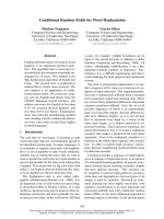
an introduction to conditional random fields for relational learning

1 An Introduction to Conditional Random
Fields for Relational Learning
Charles Sutton
Department of Computer Science
Unive rsity of Massachusetts, USA

/>Andrew McCallum
Department of Computer Science
Unive rsity of Massachusetts, USA

/>1.1 Introduction
Relational data has two characteristics: first, statistical dependencies exist between
the entities we wish to model, and second, e ach entity often has a rich set of features
that can aid classification. For example, when classifying Web documents, the
page’s text provides much information about the class label, but hyperlinks define
a relationship between pages that can improve classification [Taskar et al., 2002].
Graphical models are a natural formalism for exploiting the dependence structure
among entities. Traditionally, graphical models have been used to represent the
joint probability distribution p(y, x), where the variables y represent the attributes
of the entities that we wish to predict, and the input variables x represent our
observed knowledge about the entities. But modeling the joint distribution can
lead to difficulties when using the rich local features that can occur in relational
data, because it requires modeling the distribution p(x), which can include complex
dependencies. Modeling these dependencies among inputs can lead to intractable
models, but ignoring them can lead to reduced performance.
A solution to this problem is to directly mo del the conditional distribution p(y|x),
which is sufficient for classification. This is the approach taken by conditional ran-
dom fields [Lafferty et al., 2001]. A conditional random field is simply a conditional
distribution p(y|x) with an associated graphical structure. Because the model is
2 An Introduction to Conditional Random Fields for Relational Learning
conditional, dependencies among the input variables x do not need to be explicitly

represented, affording the use of rich, global features of the input. For example,
in natural language tasks, useful features include neighb oring words and word bi-
grams, prefixes and suffixes, capitalization, membership in domain-specific lexicons,
and semantic information from sources such as WordNet. Recently there has been
an explosion of interest in CRFs, with successful applications including text process-
ing [Taskar et al., 2002, Peng and McCallum, 2004, Settles, 2005, Sha and Pereira,
2003], bioinformatics [Sato and Sakakibara, 2005, Liu et al., 2005], and computer
vision [He et al., 2004, Kumar and Hebert, 2003].
This chapter is divided into two parts. First, we present a tutorial on current
training and inference techniques for conditional random fields. We discuss the
important special case of linear-chain CRFs, and then we generalize these to
arbitrary graphical structures. We include a brief discussion of techniques for
practical CRF implementations.
Second, we present an example of applying a general CRF to a practical relational
learning problem. In particular, we discuss the problem of information extraction,
that is, automatically building a relational database from information contained
in unstructured text. Unlike linear-chain models, general CRFs can capture long
distance dependencies between labels. For example, if the same name is mentioned
more than once in a document, all mentions probably have the same label, and it
is useful to extract them all, because each mention may contain different comple-
mentary information about the underlying entity. To represent these long-distance
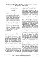
dependencies, we propose a skip-chain CRF, a model that jointly performs seg-
mentation and collective labeling of extracted mentions. On a standard problem
of extracting speaker names from seminar announcements, the skip-chain CRF has
better performance than a linear-chain CRF.
1.2 Graphical Models
1.2.1 Definitions
We consider probability distributions over sets of random variables V = X ∪ Y ,
where X is a set of input variables that we assume are observed, and Y is a set of
output variables that we wish to predict. Every variable v ∈ V takes outcomes from

a set V, which can be either continuous or discrete, although we discuss only the
discrete case in this chapter. We denote an assignment to X by x, and we denote
an assignment to a set A ⊂ X by x
A
, and similarly for Y . We use the notation
1
{x=x

}
to denote an indicator function of x which takes the value 1 when x = x

and 0 otherwise.
A graphical model is a family of probability distributions that factorize according
to an underlying graph. The main idea is to represent a distribution over a large
number of random variables by a product of lo cal functions that each depend on
only a small number of variables. Given a collection of subsets A ⊂ V , we define
1.2 Graphical Models 3
an undirected graphical model as the set of all distributions that can be written in
the form
p(x, y) =
1
Z

A
Ψ
A
(x
A
, y
A

), (1.1)
for any choice of factors F = {Ψ
A
}, where Ψ
A
: V
n
→ 
+
. (These functions are
also called local functions or compatibility functions.) We will occasionally use the
term random field to refer to a particular distribution among those defined by an
undirected model. To reiterate, we will consistently use the term model to refer to a
family of distributions, and random field (or more commonly, distribution) to refer
to a single one.
The constant Z is a normalization factor defined as
Z =

x,y

A
Ψ
A
(x
A
, y
A
), (1.2)
which ensures that the distribution sums to 1. The quantity Z, considered as a
function of the set F of factors, is called the partition function in the statistical

physic s and graphical models communities. Computing Z is intractable in general,
but much work exists on how to approximate it.
Graphically, we represent the factorization (1.1) by a factor graph [Kschischang
et al., 2001]. A factor graph is a bipartite graph G = (V, F, E) in which a variable
node v
s
∈ V is connected to a factor node Ψ
A
∈ F if v
s
is an argument to Ψ
A
. An
example of a factor graph is shown graphically in Figure 1.1 (right). In that figure,
the circles are variable nodes, and the shaded boxes are factor nodes.
In this chapter, we will assume that each local function has the form
Ψ
A
(x
A
, y
A
) = exp


k
θ
Ak
f
Ak

(x
A
, y
A
)

, (1.3)
for some real-valued parameter vector θ
A
, and for some set of feature functions or
sufficient statistics {f
Ak
}. This form ensures that the family of distributions over V
parameterized by θ is an exponential family. Much of the discussion in this chapter
actually applies to exponential families in general.
A directed graphical model, also known as a Bayesian network, is based on a directed
graph G = (V, E). A directed model is a family of distributions that factorize as:
p(y, x) =

v ∈V
p(v|π(v)), (1.4)
where π(v) are the parents of v in G. An example of a directed model is shown in
Figure 1.1 (left).
We use the term generative model to refer to a directed graphical model in which
the outputs topologically precede the inputs, that is, no x ∈ X can be a parent of
an output y ∈ Y . Essentially, a generative model is one that directly describes how
the outputs probabilistically “generate” the inputs.
4 An Introduction to Conditional Random Fields for Relational Learning
x
y

x
y
Figure 1.1 The naive Bayes classifier, as a directed model (left), and as a factor
graph (right).
1.2.2 Applications of graphical models
In this section we discuss a few applications of graphical models to natural language
processing. Although these examples are well-known, they serve both to clarify the
definitions in the previous section, and to illustrate some ideas that will arise again
in our discussion of conditional random fields. We devote special attention to the
hidden Markov model (HMM), because it is closely related to the linear-chain CRF.
1.2.2.1 Classification
First we discuss the problem of classification, that is, predicting a single class
variable y given a vector of features x = (x
1
, x
2
, . . . , x
K
). One simple way to
accomplish this is to assume that once the class label is known, all the features
are indep e ndent. The resulting classifier is called the naive Bayes classifier. It is
based on a joint probability model of the form:
p(y, x) = p(y)
K

k=1
p(x
k
|y). (1.5)
This model can be described by the directed model shown in Figure 1.1 (left). We

can also write this model as a factor graph, by defining a factor Ψ(y) = p(y), and
a factor Ψ
k
(y, x
k
) = p(x
k
|y) for each feature x
k
. This factor graph is shown in
Figure 1.1 (right).
Another well-known classifier that is naturally represented as a graphical model is
logistic regression (sometimes known as the maximum entropy classifier in the NLP
community). In statistics, this classifier is motivated by the assumption that the log
probability, log p(y|x), of each class is a linear function of x, plus a normalization
constant. This leads to the conditional distribution:
p(y|x) =
1
Z(x)
exp



λ
y
+
K

j=1
λ

y ,j
x
j



, (1.6)
where Z(x) =

y
exp{λ
y
+

K
j=1
λ
y , j
x
j
} is a normalizing constant, and λ
y
is a
bias weight that acts like log p(y) in naive Bayes. Rather than using one vector per
class, as in (1.6), we can use a different notation in which a single set of weights is
shared across all the classes. The trick is to define a set of feature functions that are
1.2 Graphical Models 5
nonzero only for a single class. To do this, the feature functions can be defined as
f
y


,j
(y, x) = 1
{y

=y }
x
j
for the feature weights and f
y

(y, x) = 1
{y

=y }
for the bias
weights. Now we can use f
k
to index each feature function f
y

,j
, and λ
k
to index
its corresponding weight λ
y

,j
. Using this notational trick, the logistic regression

model becomes:
p(y|x) =
1
Z(x)
exp

K

k=1
λ
k
f
k
(y, x)

. (1.7)
We introduce this notation because it mirrors the usual notation for conditional
random fields.
1.2.2.2 Sequence Models
Classifiers predict only a single clas s variable, but the true power of graphical
models lies in their ability to model many variables that are interdependent. In this
section, we discuss perhaps the simplest form of dependency, in which the output
variables are arranged in a sequence. To motivate this kind of model, we discuss an
application from natural language processing, the task of named-entity recognition
(NER). NER is the problem of identifying and classifying proper names in text,
including locations, such as China; people, such as George Bush; and organizations,
such as the United Nations. The named-entity recognition task is, given a sentence,
first to segment which words are part of entities, and then to classify each entity
by type (person, organization, location, and so on). The challenge of this problem
is that many named entities are too rare to appear even in a large training set, and

therefore the system must identify them based only on context.
One approach to NER is to classify each word independently as one of either
Person, Location, Organization, or Other (meaning not an entity). The
problem with this approach is that it assumes that given the input, all of the named-
entity labels are independent. In fact, the named-entity labels of neighboring words
are dependent; for example, while New York is a location, New York Times is an
organization.
This independence assumption can be relaxed by arranging the output variables in
a linear chain. This is the approach taken by the hidden Markov model (HMM)
[Rabiner, 1989]. An HMM models a sequence of observations X = {x
t
}
T
t=1
by
assuming that there is an underlying sequence of states Y = {y
t
}
T
t=1
draw n from a
finite state set S. In the named-entity example, each observation x
t
is the identity
of the word at position t, and each state y
t
is the named-entity label, that is, one
of the entity types Person, Location, Organization, and Other.
To model the joint distribution p(y, x) tractably, an HMM makes two independence
assumptions. First, it assumes that each state depends only on its immediate

predecessor, that is, each state y
t
is independent of all its ancestors y
1
, y
2
, . . . , y
t−2
given its previous state y
t−1
. Second, an HMM assumes that each observation
variable x
t
depends only on the current state y
t
. With these assumptions, we can
6 An Introduction to Conditional Random Fields for Relational Learning
specify an HMM using three probability distributions: first, the distribution p(y
1
)
over initial states; s ec ond, the transition distribution p(y
t
|y
t−1
); and finally, the
observation distribution p(x
t
|y
t
). That is, the joint probability of a s tate sequence

y and an observation sequence x factorizes as
p(y, x) =
T

t=1
p(y
t
|y
t−1
)p(x
t
|y
t
), (1.8)
where, to simplify notation, we write the initial state distribution p(y
1
) as p(y
1
|y
0
).
In natural language processing, HMMs have been used for sequence labeling tasks
such as part-of-speech tagging, named-entity recognition, and information extrac-
tion.
1.2.3 Discriminative and Generative Models
An important difference between naive Bayes and logistic regression is that naive
Bayes is generative, meaning that it is based on a model of the joint distribution
p(y, x), while logistic regression is discriminative, meaning that it is based on
a model of the conditional distribution p(y|x). In this section, we discuss the
differences between generative and discriminative modeling, and the advantages of

discriminative modeling for many tasks. For concreteness, we focus on the examples
of naive Bayes and logistic regression, but the discussion in this section actually
applies in general to the differences between generative models and conditional
random fields.
The main difference is that a conditional distribution p(y|x) does not include a
model of p(x), which is not needed for classification anyway. The difficulty in
modeling p(x) is that it often contains many highly dependent features, which
are difficult to model. For example, in named-entity recognition, an HMM relies on
only one feature, the word’s identity. But many words, es pecially proper names, will
not have occurred in the training set, so the word-identity feature is uninformative.
To label unseen words, we would like to exploit other features of a word, s uch as
its capitalization, its neighboring words, its prefixes and suffixes, its membership in
predetermined lists of people and locations, and so on.
To include interdependent features in a generative model, we have two choices: en-
hance the model to represent dependencies among the inputs, or make simplifying
independence assumptions, such as the naive Bayes assumption. The first approach,
enhancing the model, is often difficult to do while retaining tractability. For exam-
ple, it is hard to imagine how to model the dependence between the capitalization of
a word and its suffixes, nor do we particularly wis h to do so, since we always obse rve
the test sentences anyway. The second approach, adding independence assumptions
among the inputs, is problematic because it can hurt performance. For example,
although the naive Bayes classifier performs surprisingly well in document classi-
fication, it performs worse on average across a range of applications than logistic
regression [Caruana and Niculescu-Mizil, 2005].
1.2 Graphical Models 7
Logistic Regression
HMMs
Linear-chain CRFs
Naive Bayes
SEQUENCE

SEQUENCE
CONDITIONAL
CONDITIONAL
Generative directed models
General CRFs
CONDITIONAL
General
GRAPHS
General
GRAPHS
Figure 1.2 Diagram of the relationship between naive Bayes, logistic regression,
HMMs, linear-chain CRFs, generative models, and general CRFs.
Furthermore, even when naive Bayes has good classification accuracy, its prob-
ability estimates tend to be poor. To understand why, imagine training naive
Bayes on a data set in which all the features are repeated, that is, x =
(x
1
, x
1
, x
2
, x
2
, . . . , x
K
, x
K
). This will increase the confidence of the naive Bayes
probability estimate s, even though no new information has been added to the data.
Assumptions like naive Bayes can be especially problematic when we generalize

to sequence models, because inference essentially combines evidence from different
parts of the model. If probability estimates at a local level are overconfident, it
might be difficult to combine them se nsibly.
Actually, the difference in performance between naive Bayes and logistic regression
is due only to the fact that the first is generative and the second discriminative;
the two classifiers are, for discrete input, identical in all other respects. Naive Bayes
and logistic regression consider the same hypothesis space, in the sense that any
logistic regression classifier can be converted into a naive Bayes classifier with the
same decision boundary, and vic e versa. Another way of saying this is that the naive
Bayes model (1.5) defines the same family of distributions as the logistic regression
model (1.7), if we interpret it generatively as
p(y, x) =
exp {

k
λ
k
f
k
(y, x)}

˜y ,
˜
x
exp {

k
λ
k
f

k
(˜y,
˜
x)}
. (1.9)
This means that if the naive Bayes model (1.5) is trained to maximize the con-
ditional likelihood, we recover the s ame classifier as from logistic regression. Con-
versely, if the logistic regression model is interpreted generatively, as in (1.9), and is
trained to maximize the joint like lihood p(y, x), then we recover the same classifier
as from naive Bayes. In the terminology of Ng and Jordan [2002], naive Bayes and
logistic regression form a generative-discriminative pair.
The principal advantage of discriminative modeling is that it is better suited to
8 An Introduction to Conditional Random Fields for Relational Learning
including rich, overlapping features. To understand this, consider the family of naive
Bayes distributions (1.5). This is a family of joint distributions whose conditionals
all take the “logistic regression form” (1.7). But there are many other joint models,
some with complex dependencies among x, whose conditional distributions also
have the form (1.7). By modeling the conditional distribution directly, we can
remain agnostic about the form of p(x). This may explain why it has been observed
that conditional random fields tend to be more robust than generative models to
violations of their independence assumptions [Lafferty et al., 2001]. Simply put,
CRFs make independence assumptions among y, but not among x.
Another way to make the same point is due to Minka [2005]. Suppose we have a
generative model p
g
with parameters θ. By definition, this takes the form
p
g
(y, x; θ) = p
g

(y; θ)p
g
(x|y; θ). (1.10)
But we could also rewrite p
g
using Bayes rule as
p
g
(y, x; θ) = p
g
(x; θ )p
g
(y|x; θ), (1.11)
where p
g
(x; θ ) and p
g
(y|x; θ) are computed by inference, i.e., p
g
(x; θ ) =

y
p
g
(y, x; θ)
and p
g
(y|x; θ) = p
g
(y, x; θ)/p

g
(x; θ ).
Now, compare this generative model to a discriminative model over the same family
of joint distributions. To do this, we define a prior p(x) over inputs, such that p(x)
could have arisen from p
g
with some parameter setting. That is, p(x) = p
c
(x; θ

) =

y
p
g
(y, x|θ

). We combine this with a conditional distribution p
c
(y|x; θ) that
could also have arisen from p
g
, that is, p
c
(y|x; θ) = p
g
(y, x; θ)/p
g
(x; θ ). Then the
resulting distribution is

p
c
(y, x) = p
c
(x; θ

)p
c
(y|x; θ). (1.12)
By comparing (1.11) with (1.12), it can be seen that the conditional approach has
more freedom to fit the data, because it does not require that θ = θ

. Intuitively,
because the parameters θ in (1.11) are used in both the input distribution and the
conditional, a good set of parameters must represent both well, potentially at the
cost of trading off accuracy on p(y|x), the distribution we care about, for accuracy
on p(x), which we care less about.
In this section, we have discussed the relationship between naive Bayes and lo-
gistic regression in detail because it mirrors the relationship between HMMs and
linear-chain CRFs. Just as naive Bayes and logistic regression are a generative-
discriminative pair, there is a discriminative analog to hidden Markov models, and
this analog is a particular type of conditional random field, as we explain next. The
analogy between naive Bayes, logistic regression, generative models, and conditional
random fields is depicted in Figure 1.2.
1.3 Linear-Chain Conditional Random Fields 9
. . .
. . .
y
x
Figure 1.3 Graphical model of an HMM-like linear-chain CRF.

. . .
. . .
y
x
Figure 1.4 Graphical model of a linear-chain CRF in which the transition score
depends on the current observation.
1.3 Linear-Chain Conditional Random Fields
In the previous section, we have seen advantages both to discriminative modeling
and sequence modeling. So it makes sense to combine the two. This yields a linear-
chain CRF, which we describe in this section. First, in Section 1.3.1, we define linear-
chain CRFs, motivating them from HMMs. Then, we discuss parameter estimation
(Section 1.3.2) and inference (Section 1.3.3) in linear-chain CRFs.
1.3.1 From HMMs to CRFs
To motivate our introduction of linear-chain conditional random fields, we begin
by considering the conditional distribution p(y|x) that follows from the joint
distribution p(y, x) of an HMM. The key point is that this conditional distribution
is in fact a conditional random field with a particular choice of feature functions.
First, we rewrite the HMM joint (1.8) in a form that is more amenable to general-
ization. This is
p(y, x) =
1
Z
exp




t

i,j∈S

λ
ij
1
{y
t
=i}
1
{y
t−1
=j}
+

t

i∈S

o∈O
µ
oi
1
{y
t
=i}
1
{x
t
=o}




,
(1.13)
where θ = {λ
ij
, µ
oi
} are the parameters of the distribution, and can b e any real
numbers. Every HMM can be written in this form, as can be seen simply by setting
λ
ij
= log p(y

= i|y = j) and so on. Because we do not require the parameters to
be log probabilities, we are no longer guaranteed that the distribution sums to 1,
unless we explicitly enforce this by using a normalization constant Z. Despite this
added flexibility, it can be shown that (1.13) describes exactly the class of HMMs
in (1.8); we have added flexibility to the parameterization, but we have not added
any distributions to the family.
10 An Introduction to Conditional Random Fields for Relational Learning
We can write (1.13) more compactly by introducing the concept of feature functions,
just as we did for logistic regression in (1.7). Each feature function has the
form f
k
(y
t
, y
t−1
, x
t
). In order to duplicate (1.13), there needs to be one feature

f
ij
(y, y

, x) = 1
{y =i}
1
{y

=j}
for each transition (i, j) and one feature f
io
(y, y

, x) =
1
{y =i}
1
{x=o}
for each state-observation pair (i, o). Then we can write an HMM as:
p(y, x) =
1
Z
exp

K

k=1
λ
k

f
k
(y
t
, y
t−1
, x
t
)

. (1.14)
Again, equation (1.14) defines exactly the same family of distributions as (1.13),
and therefore as the original HMM equation (1.8).
The last step is to write the conditional distribution p(y|x) that results from the
HMM (1.14). This is
p(y|x) =
p(y, x)

y

p(y

, x)
=
exp


K
k=1
λ

k
f
k
(y
t
, y
t−1
, x
t
)


y

exp


K
k=1
λ
k
f
k
(y

t
, y

t−1
, x

t
)

. (1.15)
This conditional distribution (1.15) is a linear-chain CRF, in particular one that
includes features only for the current word’s identity. But many other linear-chain
CRFs use richer features of the input, such as prefixes and suffixes of the current
word, the identity of surrounding words, and so on. Fortunately, this extension
requires little change to our existing notation. We simply allow the feature functions
f
k
(y
t
, y
t−1
, x
t
) to be more general than indicator functions. This leads to the general
definition of linear-chain C RFs, which we present now.
Definition 1.1
Let Y, X be random vectors, Λ = {λ
k
} ∈ 
K
be a parameter vector, and
{f
k
(y, y

, x

t
)}
K
k=1
be a set of real-valued feature functions. Then a linear-chain
conditional random field is a distribution p(y|x) that takes the form
p(y|x) =
1
Z(x)
exp

K

k=1
λ
k
f
k
(y
t
, y
t−1
, x
t
)

, (1.16)
where Z(x) is an instance-specific normalization function
Z(x) =


y
exp

K

k=1
λ
k
f
k
(y
t
, y
t−1
, x
t
)

. (1.17)
We have just seen that if the joint p(y, x) factorizes as an HMM, then the associated
conditional distribution p(y|x) is a linear-chain CRF. This HMM-like CRF is
pictured in Figure 1.3. Other types of linear-chain CRFs are also useful, however.
For example, in an HMM, a transition from state i to state j receives the same
score, log p(y
t
= j|y
t−1
= i), regardless of the input. In a CRF, we can allow the
score of the transition (i, j) to depend on the current observation vector, simply
1.3 Linear-Chain Conditional Random Fields 11

by adding a feature 1
{y
t
=j}
1
{y
t−1
=1}
1
{x
t
=o}
. A CRF with this kind of transition
feature, which is commonly use d in text applications, is pictured in Figure 1.4.
To indicate in the definition of linear-chain CRF that each feature function can
depend on observations from any time step, we have written the observation
argument to f
k
as a vector x
t
, which should be understo od as containing all the
components of the global observations x that are needed for computing features
at time t. For example, if the CRF uses the next word x
t+1
as a feature, then the
feature vector x
t
is assumed to include the identity of word x
t+1
.

Finally, note that the normalization constant Z(x) sums over all possible state
sequences, an exp onentially large number of terms. Nevertheless, it can be computed
efficiently by forward-backward, as we explain in Section 1.3.3.
1.3.2 Parameter Estimation
In this section we discuss how to estimate the parameters θ = {λ
k
} of a linear-
chain CRF. We are given iid training data D = {x
(i)
, y
(i)
}
N
i=1
, where each x
(i)
=
{x
(i)
1
, x
(i)
2
, . . . x
(i)
T
} is a sequence of inputs, and each y
(i)
= {y
(i)

1
, y
(i)
2
, . . . y
(i)
T
} is
a sequence of the desired predictions. Thus, we have relaxed the iid assumption
within each sequence, but we still assume that distinct sequences are independent.
(In Section 1.4, we will see how to relax this assumption as well.)
Parameter estimation is typically performed by penalized maximum likelihood.
Because we are modeling the conditional distribution, the following log likelihood,
sometimes called the conditional log likelihood, is appropriate:
(θ) =
N

i=1
log p(y
(i)
|x
(i)
). (1.18)
One way to understand the conditional likelihood p(y|x; θ) is to imagine combining
it with some arbitrary prior p(x; θ

) to form a joint p(y, x). Then when we optimize
the joint log likelihood
log p(y, x) = log p(y|x; θ) + log p(x; θ


), (1.19)
the two terms on the right-hand side are decoupled, that is , the value of θ

does
not affect the optimization over θ. If we do not need to estimate p(x), then we can
simply drop the second term, which leaves (1.18).
After substituting in the CRF model (1.16) into the likelihood (1.18), we get the
following expression:
(θ) =
N

i=1
T

t=1
K

k=1
λ
k
f
k
(y
(i)
t
, y
(i)
t−1
, x
(i)

t
) −
N

i=1
log Z(x
(i)
), (1.20)
Before we discuss how to optimize this, we mention regularization. It is often the
case that we have a large number of parameters. As a measure to avoid overfitting,
we use regularization, which is a penalty on weight vectors whose norm is too
12 An Introduction to Conditional Random Fields for Relational Learning
large. A comm on choice of penalty is based on the Euclidean norm of θ and on a
regularization parameter 1/2σ
2
that determines the strength of the penalty. Then
the regularized log likelihood is
(θ) =
N

i=1
T

t=1
K

k=1
λ
k
f

k
(y
(i)
t
, y
(i)
t−1
, x
(i)
t
) −
N

i=1
log Z(x
(i)
) −
K

k=1
λ
2
k
2σ
2
. (1.21)
The notation for the regularizer is intended to suggest that regularization can also
be viewed as performing maximum a posteriori estimation of θ, if θ is assigned
a Gaussian prior with mean 0 and covariance σ
2

I. The parameter σ
2
is a free
parameter which determines how much to penalize large weights. Determining the
best regularization parameter can require a computationally-intensive parameter
sweep. Fortunately, often the accuracy of the final model does not appear to
be sensitive to changes in σ
2
, even when σ
2
is varied up to a factor of 10. An
alternative choice of regularization is to use the 
1
norm instead of the Euclidean
norm, which corresponds to an exponential prior on parameters [Goodman, 2004].
This regularizer tends to encourage sparsity in the learned parameters.
In general, the function (θ) cannot be maximized in closed form, so numerical
optimization is used. The partial derivatives of (1.21) are
∂
∂λ
k
=
N

i=1
T

t=1
f
k

(y
(i)
t
, y
(i)
t−1
, x
(i)
t
) −
N

i=1
T

t=1

y ,y

f
k
(y, y

, x
(i)
t
)p(y, y

|x
(i)

) −
K

k=1
λ
k
σ
2
.
(1.22)
The first term is the expected value of f
k
under the empirical distribution:
˜p(y, x) =
1
N
N

i=1
1
{
y=y
(i)
}
1
{
x=x
(i)
}
. (1.23)

The second term, which arises from the derivative of log Z(x), is the expectation
of f
k
under the model distribution p(y|x; θ)˜p(x). Therefore, at the unregularized
maximum likelihood solution, when the gradient is ze ro, these two expectations are
equal. This pleasing interpretation is a standard result about maximum likelihoo d
estimation in exponential families.
Now we discuss how to optimize (θ). The function (θ) is concave, which follows
from the convexity of functions of the form g(x) = log

i
exp x
i
. Convexity is
extremely helpful for parameter estimation, because it means that every local
optimum is also a global optimum. Adding regularization ensures that  is strictly
concave, which implies that it has exactly one global optimum.
Perhaps the simplest approach to optimize  is steepest ascent along the gradient
(1.22), but this requires too many iterations to be practical. Newton’s method
converges much faster because it takes into account the curvature of the likelihood,
but it requires computing the Hessian, the matrix of all second derivatives. The size
of the Hessian is quadratic in the number of parameters. Since practical applications
often use tens of thousands or even millions of parameters, even storing the full
Hessian is not practical.
1.3 Linear-Chain Conditional Random Fields 13
Instead, current techniques for optimizing (1.21) make approximate use of second-
order information. Particularly successful have been quasi-New ton methods such
as BFGS [Bertsekas, 1999], which compute an approximation to the Hessian from
only the first derivative of the objective function. A full K × K approximation to
the Hessian still requires quadratic size, however, so a limited-memory version of

BFGS is used, due to Byrd et al. [1994]. As an alternative to limited-memory BFGS,
conjugate gradient is another optimization technique that also makes approximate
use of second-order information and has been used successfully with CRFs. Either
can be thought of as a black-box optimization routine that is a drop-in replacement
for vanilla gradient ascent. When such second-order methods are used, gradient-
based optimization is much faster than the original approaches based on iterative
scaling in Lafferty et al. [2001], as shown experimentally by several authors [Sha
and Pereira, 2003, Wallach, 2002, Malouf, 2002, Minka, 2003].
Finally, it is important to remark on the computational cost of training. Both the
partition function Z(x) in the likelihood and the marginal distributions p(y
t
, y
t−1
|x)
in the gradient can be computed by forward-backward, which uses computational
complexity O(T M
2
). However, each training instance will have a different partition
function and marginals, so we need to run forward-backward for each training
instance for each gradient computation, for a total training cost of O(TM
2
NG),
where N is the number of training examples, and G the number of gradient
computations required by the optimization procedure. For many data sets, this
cost is reasonable, but if the number of states is large, or the number of training
sequences is very large, then this can become expensive. For example, on a standard
named-entity data set, with 11 labels and 200,000 words of training data, CRF
training finishes in under two hours on current hardware. However, on a part-of-
speech tagging data set, with 45 labels and one million words of training data, CRF
training requires over a week.

1.3.3 Inference
There are two common inference problems for CRFs. First, during training, com-
puting the gradient requires marginal distributions for each edge p(y
t
, y
t−1
|x), and
computing the likelihood requires Z(x). Second, to label an unseen instance, we
compute the most likely (Viterbi) labeling y
∗
= arg max
y
p(y|x). In linear-chain
CRFs, both inference tasks can be performed efficiently and exactly by variants
of the standard dynamic-programming algorithms for HMMs. In this se ction, we
briefly review the HMM algorithms, and extend them to linear-chain CRFs. These
standard inference algorithms are described in more detail by Rabiner [1989].
First, we introduce notation which will simplify the forward-backward recursions.
An HMM can be viewed as a factor graph p(y, x) =

t
Ψ
t
(y
t
, y
t−1
, x
t
) where Z = 1,

and the factors are defined as:
Ψ
t
(j, i, x)
def
= p(y
t
= j|y
t−1
= i)p(x
t
= x|y
t
= j). (1.24)
14 An Introduction to Conditional Random Fields for Relational Learning
If the HMM is viewed as a weighted finite state machine, then Ψ
t
(j, i, x) is the
weight on the transition from state i to state j when the current observation is x.
Now, we review the HMM forward algorithm, which is used to compute the
probability p(x) of the observations. The idea behind forward-backward is to first
rewrite the naive summation p(x) =

y
p(x, y) using the distributive law:
p(x) =

y
T


t=1
Ψ
t
(y
t
, y
t−1
, x
t
) (1.25)
=

y
T

y
T−1
Ψ
T
(y
T
, y
T−1
, x
T
)

y
T−2
Ψ

T−1
(y
T−1
, y
T−2
, x
T−1
)

y
T−3
· · · (1.26)
Now we observe that each of the intermediate sums is reused many times during
the computation of the outer sum, and so we can save an exponential amount of
work by caching the inner sums.
This leads to defining a set of forward variables α
t
, each of which is a vector of size
M (where M is the number of states) which stores one of the intermediate sums.
These are defined as:
α
t
(j)
def
= p(x
1 t
, y
t
= j) (1.27)
=


y
1 t−1
Ψ
t
(j, y
t−1
, x
t
)
t−1

t

=1
Ψ
t

(y
t

, y
t

−1
, x
t

), (1.28)
where the summation over y

1 t−1
ranges over all assignments to the sequence
of random variables y
1
, y
2
, . . . , y
t−1
. The alpha values can be computed by the
recursion
α
t
(j) =

i∈S
Ψ
t
(j, i, x
t
)α
t−1
(i), (1.29)
with initialization α
1
(j) = Ψ
1
(j, y
0
, x
1

). (Recall that y
0
is the fixed initial state of
the HMM.) It is easy to see that p(x) =

y
T
α
T
(y
T
) by repeatedly substituting the
recursion (1.29) to obtain (1.26). A formal proof would use induction.
The backward recursion is exactly the same, except that in (1.26), we push in the
summations in reverse order. This results in the definition
β
t
(i)
def
= p(x
t+1 T
|y
t
= i) (1.30)
=

y
t+1 T
T


t

=t+1
Ψ
t

(y
t

, y
t

−1
, x
t

), (1.31)
and the recursion
β
t
(i) =

j∈S
Ψ
t+1
(j, i, x
t+1
)β
t+1
(j), (1.32)

which is initialized β
T
(i) = 1. Analogously to the forward case, we can compute
p(x) using the backward variables as p(x) = β
0
(y
0
)
def
=

y
1
Ψ
1
(y
1
, y
0
, x
1
)β
1
(y
1
).
1.3 Linear-Chain Conditional Random Fields 15
By combining results from the forward and backward recursions, we can compute
the marginal distributions needed for the gradient (1.22). Applying the distributive
law again, we see that

p(y
t−1
, y
t
|x) = Ψ
t
(y
t
, y
t−1
, x
t
)



y
1 t−2
t−1

t

=1
Ψ
t

(y
t

, y

t

−1
, x
t

)





y
t+1 T
T

t

=t+1
Ψ
t

(y
t

, y
t

−1
, x

t

)


, (1.33)
which can be computed from the forward and backward recursions as
p(y
t−1
, y
t
|x) ∝ α
t−1
(y
t−1
)Ψ
t
(y
t
, y
t−1
, x
t
)β
t
(y
t
). (1.34)
Finally, to compute the globally most probable assignment y
∗

= arg max
y
p(y|x),
we obse rve that the trick in (1.26) still works if all the summations are replaced by
maximization. This yields the Viterbi recursion:
δ
t
(j) = max
i∈S
Ψ
t
(j, i, x
t
)δ
t−1
(i) (1.35)
Now that we have described the forward-backward and Viterbi algorithms for
HMMs, the generalization to linear-chain CRFs is fairly straightforward. The
forward-backward algorithm for linear-chain CRFs is identical to the HMM version,
except that the transition weights Ψ
t
(j, i, x
t
) are defined differently. We observe that
the CRF model (1.16) can be rewritten as:
p(y|x) =
1
Z(x)
T


t=1
Ψ
t
(y
t
, y
t−1
, x
t
), (1.36)
where we define
Ψ
t
(y
t
, y
t−1
, x
t
) = exp


k
λ
k
f
k
(y
t
, y

t−1
, x
t
)

. (1.37)
With that definition, the forward recursion (1.29), the backward recursion (1.32),
and the Viterbi recursion (1.35) can be used unchanged for linear-chain CRFs.
Instead of computing p(x) as in an HMM, in a CRF the forward and backward
recursions compute Z(x).
A final inference task that is useful in some applications is to compute a marginal
probability p(y
t
, y
t+1
, . . . y
t+k
|x) over a range of nodes. For example, this is useful
for measuring the model’s confidence in its predicted labeling over a segment of
input. This marginal probability can be computed efficiently using constrained
forward-backward, as described by Culotta and McCallum [2004].
16 An Introduction to Conditional Random Fields for Relational Learning
1.4 CRFs in General
In this section, we define CRFs with general graphical structure, as they were
introduced originally [Lafferty et al., 2001]. Although initial applications of CRFs
used linear chains, there have been many later applications of CRFs with more
general graphical structures. Such structures are especially useful for relational
learning, because they allow relaxing the iid assumption among entities. Also,
although CRFs have typically been used for across-network classification, in which
the training and testing data are assumed to be independent, we will see that CRFs

can be used for within-network classification as well, in which we model probabilistic
dependencies between the training and testing data.
The generalization from linear-chain CRFs to general CRFs is fairly straightfor-
ward. We simply move from using a linear-chain factor graph to a more general
factor graph, and from forward-backward to more general (perhaps approximate)
inference algorithms.
1.4.1 Model
First we present the general definition of a c onditional random field.
Definition 1.2
Let G be a factor graph over Y . Then p(y|x) is a conditional random field if for
any fixed x, the distribution p(y|x) factorizes according to G.
Thus, every conditional distribution p(y|x) is a CRF for some, perhaps trivial,
factor graph. If F = {Ψ
A
} is the set of factors in G, and each factor takes the
exponential family form (1.3), then the conditional distribution can be written as
p(y|x) =
1
Z(x)

Ψ
A
∈G
exp



K(A)

k=1

λ
Ak
f
Ak
(y
A
, x
A
)



. (1.38)
In addition, practical models rely extensively on parameter tying. For exam-
ple, in the linear-chain case, often the same weights are used for the factors
Ψ
t
(y
t
, y
t−1
, x
t
) at each time step. To denote this, we partition the factors of G
into C = {C
1
, C
2
, . . . C
P

}, where each C
p
is a clique template whose parameters are
tied. This notion of clique template generalizes that in Taskar et al. [2002], Sutton
et al. [2004], and Richardson and Domingos [2005]. Each clique tem plate C
p
is a
set of factors which has a corresponding set of sufficient statistics {f
pk
(x
p
, y
p
)} and
parameters θ
p
∈ 
K(p)
. Then the CRF can be written as
p(y|x) =
1
Z(x)

C
p
∈C

Ψ
c
∈C

p
Ψ
c
(x
c
, y
c
; θ
p
), (1.39)
1.4 CRFs in General 17
where each factor is parameterized as
Ψ
c
(x
c
, y
c
; θ
p
) = exp



K(p)

k=1
λ
pk
f

pk
(x
c
, y
c
)



, (1.40)
and the normalization function is
Z(x) =

y

C
p
∈C

Ψ
c
∈C
p
Ψ
c
(x
c
, y
c
; θ

p
). (1.41)
For example, in a linear-chain conditional random field, typically one clique tem-
plate C = {Ψ
t
(y
t
, y
t−1
, x
t
)}
T
t=1
is used for the entire network.
Several special cases of conditional random fields are of particular interest. First,
dynamic conditional random fields [Sutton et al., 2004] are sequence models which
allow multiple lab els at each time step, rather than single labels as in linear-chain
CRFs. Second, relational Markov networks [Taskar et al., 2002] are a type of general
CRF in which the graphical structure and parameter tying are determined by an
SQL-like syntax. Finally, Markov logic networks [Richardson and Domingos, 2005,
Singla and Domingos, 2005] are a type of probabilistic logic in which there are
parameters for each first-order rule in a knowledge base .
1.4.2 Applications of CRFs
CRFs have been applied to a variety of domains, including text processing, com-
puter vision, and bioinformatics. In this section, we discuss several applications,
highlighting the different graphical structures that occur in the literature.
One of the first large-scale applications of CRFs was by Sha and Pereira [2003], who
matched state-of-the-art performance on segmenting noun phrases in text. Since
then, linear-chain CRFs have been applied to many problems in natural language

processing, including named-entity recognition [McCallum and Li, 2003], feature
induction for NER [McCallum, 2003], identifying protein names in biology abstracts
[Settles, 2005], segmenting addresses in Web pages [Culotta et al., 2004], finding
semantic roles in text [Roth and Yih, 2005], identifying the sources of opinions [Choi
et al., 2005], Chinese word segmentation [Peng et al., 2004], Japanese morphological
analysis [Kudo et al., 2004], and many others.
In bioinformatics, CRFs have be en applied to RNA structural alignment [Sato and
Sakakibara, 2005] and protein structure prediction [Liu et al., 2005]. Semi-Markov
CRFs [Sarawagi and Cohen, 2005] add somewhat more flexibility in choosing
features, which may be useful for certain tasks in information extraction and
especially bioinformatics.
General CRFs have also been applied to several tasks in NLP. One promising
application is to performing multiple labeling tasks simultaneously. For example,
Sutton et al. [2004] show that a two-level dynamic CRF for part-of-speech tagging
and noun-phrase chunking performs better than solving the tasks one at a time.
Another application is to multi-label classification, in which each instance can
18 An Introduction to Conditional Random Fields for Relational Learning
have multiple class labels. Rather than learning an independent classifier for each
category, Ghamrawi and McCallum [2005] present a CRF that learns dependencies
between the categories, resulting in improved classification performance. Finally, the
skip-chain CRF, which we present in Section 1.5, is a general CRF that represents
long-distance dependencies in information extraction.
An interesting graphical CRF structure has been applied to the problem of proper-
noun coreference, that is, of determining which mentions in a document, such as
Mr. President and he, refer to the same underlying entity. McCallum and Wellner
[2005] learn a distance metric between mentions using a fully-connected conditional
random field in which inference corresp onds to graph partitioning. A similar model
has been used to segment handwritten characters and diagrams [Cowans and
Szummer, 2005, Qi et al., 2005].
In some applications of CRFs, efficient dynamic programs exist even though the

graphical model is difficult to specify. For example, McCallum et al. [2005] learn
the parameters of a string-edit model in order to discriminate between matching
and nonmatching pairs of strings. Also, there is work on using CRFs to learn
distributions over the derivations of a grammar [Riezler et al., 2002, Clark and
Curran, 2004, Sutton, 2004, Viola and Narasimhan, 2005]. A potentially useful
unifying framework for this type of model is provided by case-factor diagrams
[McAllester et al., 2004].
In copmputer vision, several authors have used grid-shaped CRFs [He et al., 2004,
Kumar and Hebert, 2003] for labeling and segmenting images. Also, for recognizing
objects, Quattoni et al. [2005] use a tree-shaped CRF in which latent variables are
designed to recognize characteristic parts of an object.
1.4.3 Parameter Estimation
Parameter estimation for general CRFs is essentially the same as for linear-chains,
except that computing the model expectations requires more general inference
algorithms. First, we discuss the fully-observed case, in which the training and
testing data are independent, and the training data is fully observed. In this case
the conditional log likelihood is given by
(θ) =

C
p
∈C

Ψ
c
∈C
p
K(p)

k=1

λ
pk
f
pk
(x
c
, y
c
) − log Z(x). (1.42)
It is worth noting that the equations in this section do not explicitly sum over
training instances, because if a particular application happens to have iid training
instances, they can be represented by disconnected components in the graph G.
The partial derivative of the log likelihood with respect to a parameter λ
pk
associ-
ated with a clique template C
p
is
∂
∂λ
pk
=

Ψ
c
∈C
p
f
pk
(x

c
, y
c
) −

Ψ
c
∈C
p

y

c
f
pk
(x
c
, y

c
)p(y

c
|x). (1.43)
1.4 CRFs in General 19
The function (θ) has many of the same properties as in the linear-chain case.
First, the zero-gradient conditions can be interpreted as requiring that the suf-
ficient statistics F
pk
(x, y) =


Ψ
c
f
pk
(x
c
, y
c
) have the same expectations under
the empirical distribution and under the model distribution. Second, the function
(θ) is concave, and can be efficiently maximized by second-order techniques such
as conjugate gradient and L-BFGS. Finally, regularization is used just as in the
linear-chain case.
Now, we discuss the case of within-network classification, where there are depen-
dencies between the training and testing data. That is, the random variables y are
partitioned into a set y
tr
that is observed during training and a set y
tst
that is
unobserve d during training. It is assumed that the graph G contains connections
between y
tr
and y
tst
.
Within-network classification can be viewed as a kind of latent variable problem,
in which certain variables, in this case y
tst

, are not observed in the training data.
It is more difficult to train CRFs with latent variables, because optimizing the
likelihood p(y
tr
|x) requires marginalizing out the latent variables y
tst
. Because of
this difficultly, the original work on CRFs focused on fully-observed training data,
but recently there has been increasing interest in training latent-variable CRFs
[Quattoni et al., 2005, McCallum et al., 2005].
Supp ose we have a conditional random field with inputs x in which the output
variables y are observed in the training data, but we have additional variables w
that are latent, so that the CRF has the form
p(y, w|x) =
1
Z(x)

C
p
∈C

Ψ
c
∈C
p
Ψ
c
(x
c
, w

c
, y
c
; θ
p
). (1.44)
The objective function to maximize during training is the marginal likelihood
(θ) = log p(y|x) = log

w
p(y, w|x). (1.45)
The first question is how e ven to compute the marginal likelihood (θ), because if
there are many variables w, the sum cannot be computed directly. The key is to
realize that we need to compute log

w
p(y, w|x) not for any possible assignment
y, but only for the particular assignment that o c curs in the training data. This
motivates taking the original CRF (1.44), and clamping the variables Y to their
observed values in the training data, yielding a distribution over w:
p(w|y, x) =
1
Z(y, x)

C
p
∈C

Ψ
c

∈C
p
Ψ
c
(x
c
, w
c
, y
c
; θ
p
), (1.46)
where the normalization factor is
Z(y, x) =

w

C
p
∈C

Ψ
c
∈C
p
Ψ
c
(x
c

, w
c
, y
c
; θ
p
). (1.47)
This new normalization constant Z(y, x) can be computed by the same inference
20 An Introduction to Conditional Random Fields for Relational Learning
algorithm that we use to compute Z(x). In fact, Z(y, x) is easier to compute,
because it sums only over w, while Z(x) sums over both w and y. Graphically, this
amounts to saying that clamping the variables y in the graph G can simplify the
structure among w.
Once we have Z(y, x), the marginal likeliho od can be computed as
p(y|x) =
1
Z(x)

w

C
p
∈C

Ψ
c
∈C
p
Ψ
c

(x
c
, w
c
, y
c
; θ
p
) =
Z(y, x)
Z(x)
. (1.48)
Now that we have a way to compute , we discuss how to maximize it with respect
to θ. Maximizing (θ) can be difficult because  is no longer convex in general
(intuitively, log-sum-exp is convex, but the difference of two log-sum-exp functions
might not be), so optimization procedures are typically guaranteed to find only local
maxima. Whatever optimization technique is used, the model parameters must be
carefully initialized in order to reach a good local maximum.
We discuss two different ways to maximize : directly using the gradient, as in
Quattoni et al. [2005]; and using EM, as in McCallum et al. [2005]. To maximize 
directly, we need to calculate its gradient. The simplest way to do this is to use the
following fact. For any function f(λ), we have
df
dλ
= f(λ)
d log f
dλ
, (1.49)
which can be seen by applying the chain rule to log f and rearranging. Applying
this to the marginal likelihood (Λ) = log


w
p(y, w|x) yields
∂
∂λ
pk
=
1

w
p(y, w|x)

w
∂
∂λ
pk

p(y, w|x)

(1.50)
=

w
p(w|y, x)
∂
∂λ
pk

log p(y, w|x)


. (1.51)
This is the expectation of the fully-observed gradient, where the expectation is
taken over w. This expression simplifies to
∂
∂λ
pk
=

Ψ
c
∈C
p

w

c
p(w

c
|y, x)f
k
(y
c
, x
c
, w

c
) −


Ψ
c
∈C
p

w

c
,y

c
p(w

c
, y

c
|x
c
)f
k
(y

c
, x
c
, w

c
).

(1.52)
This gradient requires computing two different kinds of marginal probabilities.
The first term contains a marginal probability p(w

c
|y, x), which is exactly a
marginal distribution of the clamped CRF (1.46). The second term contains a
different marginal p(w

c
, y

c
|x
c
), which is the same marginal probability required
in a fully-observed CRF. Once we have computed the gradient,  can be maximized
by standard techniques such as conjugate gradient. In our experience, conjugate
gradient tolerates violations of convexity better than limited-memory BFGS, so it
may be a better choice for latent- variable CRFs .
Alternatively,  can be optimized using expectation maximization (EM). At each
1.4 CRFs in General 21
iteration j in the EM algorithm, the current parameter vector θ
(j)
is updated as
follows . First, in the E-step, an auxiliary function q(w) is computed as q (w) =
p(w|y, x; θ
(j)
). Second, in the M-step, a new parameter vector θ
(j+1)

is chosen as
θ
(j+1)
= arg max
θ


w

q(w

) log p(y , w

|x; θ

). (1.53)
The direct maximization algorithm and the EM algorithm are strikingly similar.
This can be seen by substituting the definition of q into (1.53) and taking deriva-
tives. The gradient is almost identical to the direct gradient (1.52). The only dif-
ference is that in EM, the distribution p(w|y, x) is obtained from a previous, fixed
parameter setting rather than from the argument of the maximization. We are un-
aware of any empirical comparison of EM to direct optimization for latent-variable
CRFs.
1.4.4 Inference
In general CRFs, just as in the linear-chain case, gradient-based training requires
computing marginal distributions p(y
c
|x), and testing re quires computing the most
likely assignment y
∗

= arg max
y
p(y|x). This can be accomplished using any
inference algorithm for graphical models. If the graph has small treewidth, then the
junction tree algorithm can be used to exactly compute the marginals, but because
both inference problems are NP-hard for general graphs, this is not always possible.
In such cases, approximate inference must be used to compute the gradient. In this
section, we mention various approximate inference algorithms that have been used
successfully with CRFs. Detailed discussion of these are beyond the scope of this
tutorial.
When choosing an inference algorithm to use within CRF training, the important
thing to understand is that it will be invoked repeatedly, once for each time that
the gradient is computed. For this reason, sampling-based approaches which may
take many iterations to converge, such as Markov chain Monte Carlo, have not
been popular, although they might be appropriate in some circumstances. Indeed,
contrastive divergence [Hinton, 2000], in which an MCMC sampler is run for only
a few samples, has been successfully applied to CRFs in vision [He et al., 2004].
Because of their computational efficiency, variational approaches have been most
popular for CRFs. Several authors [Taskar et al., 2002, Sutton et al., 2004] have
used loopy belief propagation. Belief propagation is an exact inference algorithm for
trees which generalizes the forward-backward. Although the generalization of the
forward-backward recursions, which are called message updates, are neither exact
nor even guaranteed to converge if the model is not a tree, they are still well-defined,
and they have been empirically successful in a wide variety of domains, including
text processing, vision, and error-correcting codes. In the past five years, there has
been much theoretical analysis of the algorithm as well. We refer the reader to
Yedidia et al. [2004] for more information.
22 An Introduction to Conditional Random Fields for Relational Learning
1.4.5 Discussion
This s ec tion contains miscellaneous remarks about CRFs. First, it is easily seen

that logistic regression model (1.7) is a conditional random field with a single
output variable. Thus, CRFs can be viewed as an extension of logistic regression
to arbitrary graphical structures.
Although we have emphasized the view of a CRF as a model of the conditional
distribution, one could view it as an objective function for parameter estimation of
joint distributions. As such, it is one objective among many, including generative
likelihood, pseudolikelihood [Besag, 1977], and the maximum-margin objective
[Taskar et al., 2004, Altun et al., 2003]. Another related discriminative technique for
structured models is the averaged perceptron, which has been especially popular in
the natural language community [Collins, 2002], in large part because of its ease of
implementation. To date, there has been little careful comparison of these, especially
CRFs and max-margin approaches, across different structures and domains.
Give n this view, it is natural to imagine training directed models by conditional
likelihood, and in fact this is commonly done in the speech community, where it is
called maximum mutual information training. However, it is no easier to maximize
the conditional likelihood in a directed model than an undirected model, because in
a directed model the conditional likelihood requires computing log p(x), which plays
the same role as Z(x) in the CRF likelihood. In fact, training is more complex in a
directed model, because the model parameters are constrained to be probabilities—
constraints which can make the optimization problem more difficult. This is in stark
contrast to the joint likelihood, which is much easier to compute for directed models
than undirected models (although recently se veral efficient parameter estimation
techniques have been proposed for undirected factor graphs, such as Abbeel et al.
[2005] and Wainwright et al. [2003]).
1.4.6 Implementation Concerns
There are a few implementation techniques that can help both training time and
accuracy of CRFs, but are not always fully discussed in the literature. Although
these apply especially to language applications, they are also useful more generally.
First, when the predicted variables are discrete, the features f
pk

are ordinarily
chosen to have a particular form:
f
pk
(y
c
, x
c
) = 1
{y
c
=
˜
y
c
}
q
pk
(x
c
). (1.54)
In other words, each feature is nonzero only for a single output configuration
˜
y
c
, but
as long as that constraint is met, then the feature value depends only on the input
observation. Essentially, this means that we can think of our features as depending
only on the input x
c

, but that we have a separate set of weights for each output
configuration. This feature representation is also computationally efficient, because
computing each q
pk
may involve nontrivial text or image processing, and it need be
1.4 CRFs in General 23
evaluated only once for every feature that uses it. To avoid confusion, we refer to
the functions q
pk
(x
c
) as observation functions rather than as features. Examples of
observation functions are “word x
t
is capitalized” and “word x
t
ends in ing”.
This representation can lead to a large number of features, which can have signifi-
cant memory and time requirements. For example, to match state-of-the-art results
on a standard natural language task, Sha and Pereira [2003] use 3.8 million features.
Not all of these features are ever nonzero in the training data. In particular, some
observation functions q
pk
are nonzero only for certain output configurations. This
point can be confusing: One might think that such features can have no effect on
the likelihood, but actually they do affect Z(x), so putting a negative we ight on
them can improve the likelihood by making wrong answers less likely. In order to
save memory, however, sometimes these unsupported features, that is, those which
never o c cur in the training data, are removed from the model. In practice, however,
including unsupported features typically results in better accuracy.

In order to get the benefits of unsupported features with less memory, we have had
success with an ad hoc technique for selecting only a few unsupported features. The
main idea is to add unsupported features only for likely paths, as follows: first train
a CRF without any unsupported features, stopping after only a few iterations; then
add unsupported features f
pk
(y
c
, x
c
) for cases where x
c
occurs in the training data,
and p(y
c
|x) > . McCallum [2003] presents a more principled method of feature
selection for CRFs.
Second, if the observations are categorical rather than ordinal, that is, if they are
discrete but have no intrinsic order, it is important to convert them to binary
features. For example, it makes sense to learn a linear weight on f
k
(y, x
t
) when f
k
is 1 if x
t
is the word dog and 0 otherwise, but not when f
k
is the integer index

of word x
t
in the text’s vocabulary. Thus, in text applications, CRF features are
typically binary; in other application areas, such as vision and speech, they are
more commonly real-valued.
Third, in language applications, it is sometimes helpful to include redundant factors
in the model. For example, in a linear-chain CRF, one may choose to include both
edge factors Ψ
t
(y
t
, y
t−1
, x
t
) and variable factors Ψ
t
(y
t
, x
t
). Although one could
define the same family of distributions using only edge factors, the redundant node
factors provide a kind of backoff, which is useful when there is too little data.
In language applications, there is always too little data, even when hundreds of
thousands of words are available.
Finally, often the probabilities involved in forward-backward and belief propagation
become too small to be represented within numerical precision. There are two
standard approaches to this common problem. One approach is to normalize each
of the vectors α

t
and β
t
to sum to 1, thereby magnifying small values. A second
approach is to perform computations in the logarithmic domain, e.g., the forward
recursion becomes
log α
t
(j) =

i∈S

log Ψ
t
(j, i, x
t
) + log α
t−1
(i)

, (1.55)
24 An Introduction to Conditional Random Fields for Relational Learning
where ⊕ is the operator a ⊕ b = log(e
a
+ e
b
). At first, this does not seem much of
an improvement, since numerical precision is lost when computing e
a
and e

b
. But
⊕ can be computed as
a ⊕ b = a + log(1 + e
b−a
) = b + log(1 + e
a−b
), (1.56)
which can be much more numerically stable, particularly if we pick the version of
the identity with the smaller exponent. CRF implementations often use the log-
space approach because it makes computing Z(x) more convenient, but in some
applications, the computational expense of taking logarithms is an issue, making
normalization preferable.
1.5 Skip-Chain CRFs
In this section, we present a case study of applying a general CRF to a practical
natural language problem. In particular, we consider a problem in information
extraction, the task of building a database automatically from unstructured text.
Recent work in extraction has often used sequence models, such as HMMs and
linear-chain CRFs, which model dependencies only between neighboring labels, on
the assumption that those dependencies are the strongest.
But sometimes it is important to model certain kinds of long-range dependencies
between entities. One important kind of dependency within information extraction
occurs on repeated mentions of the same field. When the same entity is mentioned
more than once in a document, such as Robert Booth, in many cases all mentions
have the same label, such as Seminar-Speaker. We can take advantage of this
fact by favoring lab elings that treat repeated words identically, and by combining
features from all occurrences so that the extraction decision can be made based on
global information. Furthermore, identifying all mentions of an entity can be useful
in itself, because each mention might contain different useful information. However,
most extraction systems, whether probabilistic or not, do not take advantage of

this dependency, instead treating the separate mentions independently.
To perform collective labeling, we need to represent dependencies between distant
terms in the input. But this reveals a general limitation of sequence models,
whether generatively or discriminatively trained. Sequence m odels make a Markov
assumption among labels, that is, that any label y
t
is independent of all previous
labels given its immediate predecessors y
t−k
. . . y
t−1
. This represents dependence
only between nearby nodes—for example, between bigrams and trigrams—and
cannot represent the higher-order dependencies that arise when identical words
occur throughout a document.
To relax this assumption, we introduce the skip-chain CRF, a conditional model
that collectively segments a document into mentions and classifies the mentions by
entity type, while taking into account probabilistic dependencies between distant
mentions. These dependencies are represented in a skip-chain model by augmenting
1.5 Skip-Chain CRFs 25
x
t
x
t+1
x
t-1
y
t
y
t+1

y
t-1
John GreenSenator
x
t+101
y
t+101
x
t+100
y
t+100


Green
.
x
t+101
y
t+101
ran


Figure 1.5 Graphical representation of a skip-chain CRF. Identical words are
connected because they are likely to have the same label.
w
t
= w
w
t
matches [A-Z][a-z]+

w
t
matches [A-Z][A-Z]+
w
t
matches [A-Z]
w
t
matches [A-Z]+
w
t
matches [A-Z]+[a-z]+[A-Z]+[a-z]
w
t
app e ars in list of first names,
last names, honorifics, etc.
w
t
app e ars to be part of a time followed by a dash
w
t
app e ars to be part of a time preceded by a dash
w
t
app e ars to be part of a date
T
t
= T
q
k

(x, t + δ) for all k and δ ∈ [−4, 4]
Table 1.1 Input features q
k
(x, t) for the seminars data. In the above w
t
is the word
at position t, T
t
is the POS tag at position t, w ranges over all words in the training
data, and T ranges over all part-of-speech tags returned by the Brill tagger. The
“appears to be” features are based on hand-designed re gular expressions that can
span several tokens.
a linear-chain CRF with factors that depend on the labels of distant but similar
words. This is shown graphically in Figure 1.5.
Even though the limitations of n-gram models have been widely recognized within
natural language processing, long-distance dependencies are difficult to represent
in generative models, because full n-gram models have too many parameters if n
is large. We avoid this problem by selecting which skip edges to include based on
the input string. This kind of input-specific dependence is difficult to represent in
a generative model, because it makes generating the input more complicated. In
other words, conditional models have been popular because of their flexibility in
allowing overlapping features; skip-chain CRFs take advantage of their flexibility
in allowing input-specific model structure.