kernel methods and svm's

1
Machine Learning 10-701
Tom M. Mitchell
Machine Learning Department
Carnegie Mellon University
April 7, 2011
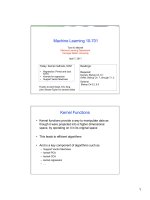
Today: Kernel methods, SVM
•  Regression: Primal and dual
forms
•  Kernels for regression
•  Support Vector Machines
Readings:
Required:
Kernels: Bishop Ch. 6.1
SVMs: Bishop Ch. 7, through 7.1.2
Optional:
Bishop Ch 6.2, 6.3
Thanks to Aarti Singh, Eric Xing,
John Shawe-Taylor for several slides
Kernel Functions
•  Kernel functions provide a way to manipulate data as
though it were projected into a higher dimensional
space, by operating on it in its original space
•  This leads to efficient algorithms
•  And is a key component of algorithms such as
–  Support Vector Machines
–  kernel PCA
–  kernel CCA
–  kernel regression
–  …
2

Linear Regression
Wish to learn f: X  Y, where X=<X
1
, … X
n
>, Y real-valued
Learn
where
Linear Regression
Wish to learn where
Learn
where
here the l
th
row of X is the l
th
training example x
Tl
and

3
Vectors, Data Points, Inner Products
Consider
where
for any two vectors, their dot product (aka inner product) is equal to product of
their lengths, times the cosine of angle between them.
Linear Regression: Primal Form
Learn
where
solve by taking derivative wrt w, setting to zero…

so:
4
Aha!
Learn
where
solution:
But notice w lies in the space spanned by training examples
(why?)
Linear Regression: Dual Form
Primal form:
Learn
Solution:
Dual form: use fact that
Learn
Solution:
5
[slide from John Shawe-Taylor]
[slide from John Shawe-Taylor]
6
[slide from John Shawe-Taylor]
[slide from John Shawe-Taylor]
7
Kernel functions
Original space Projected space
(higher dimensional)
Example: Quadratic Kernel
Suppose we have data originally in 2D, but project it into 3D using
But we can use the following kernel function to calculate inner products
in the projected 3D space, in terms of operations in the 2D space
this converts our original linear regression into quadratic regression!

And use it to train and apply our regression function, never leaving 2D space
8
[slide from John Shawe-Taylor]
Implications of the “Kernel Trick”
Some Common Kernels
•  Polynomials of degree d
•  Polynomials of degree up to d
•  Gaussian/Radial kernels (polynomials of all orders –
projected space has infinite dimension)
•  Sigmoid
9
Which Functions Can Be Kernels?
•  not all functions
•  for some definitions of k(x
1
,x
2
) there is no corresponding
projection ϕ(x)
•  Nice theory on this, including how to construct new
kernels from existing ones
•  Initially kernels were defined over data points in
Euclidean space, but more recently over strings, over
trees, over graphs, …
•  Some of this covered in 10-702
Kernels : Key Points
•  Many learning tasks are framed as optimization problems
•  Primal and Dual formulations of optimization problems
•  Dual version framed in terms of dot products between x’s
•  Kernel functions k(x,y) allow calculating dot products

<Φ(x),Φ(y)> without bothering to project x into Φ(x)
•  Leads to major efficiencies, and ability to use very high
dimensional (virtual) feature spaces
10
Kernel Based Classifiers
Simple Kernel Based Classifier
[slide from John Shawe-Taylor]
11
Linear classifiers – which line is better?
12
Pick the one with the largest margin!
Parameterizing the decision boundary
w
T
x + b = 0
w
T
x + b > 0
w
T
x + b < 0
Labels:
13
Parameterizing the decision boundary
w
T
x + b = 0
w
T
x + b > 0

w
T
x + b < 0
Labels:
Maximizing the margin
margin = γ = a/‖w‖"
w
T
x + b = 0
w
T
x + b = a
w
T
x + b = -a
γ"
γ"
Margin = Distance of
closest examples
from the decision line/
hyperplane
14
Maximizing the margin
margin = γ = a/‖w‖"
w
T
x + b = 0
w
T
x + b = a

w
T
x + b = -a
γ"
γ"
max γ = a/‖w‖"
w,b
s.t. (w
T
x
j
+b) y
j
≥ a ∀j
Note: ‘a’ is arbitrary (can normalize
equations by a)
Margin = Distance of
closest examples
from the decision line/
hyperplane
Support Vector Machine
w
T
x + b = 0
w
T
x + b = a
w
T
x + b = -a

γ"
γ"
min w
T
w"
s.t. (w
T
x
j
+b) y
j
≥ 1 ∀j
w,b
Solve efficiently by quadratic
programming (QP)
–  Well-studied solution
algorithms
Linear hyperplane defined
by “support vectors”