- Trang chủ >>
- Khoa Học Tự Nhiên >>
- Vật lý
lindell i. differential forms in electromagnetics (wiley,2004)
Bạn đang xem bản rút gọn của tài liệu. Xem và tải ngay bản đầy đủ của tài liệu tại đây (1.51 MB, 262 trang )
Differential Forms in
Electromagnetics
Ismo V. Lindell
Helsinki University of Technology, Finland
IEEE Antennas & Propagation Society, Sponsor
A JOHN WILEY & SONS, INC., PUBLICATION
IEEE PRESS
Copyright © 2004 by the Institute of Electrical and Electronic Engineers. All rights reserved.
Published simultaneously in Canada.
No part of this publication may be reproduced, stored in a retrieval system or transmitted in any form or
by any means, electronic, mechanical, photocopying, recording, scanning or otherwise, except as
permitted under Section 107 or 108 of the 1976 United States Copyright Act, without either the prior
written permission of the Publisher, or authorization through payment of the appropriate per-copy fee to
the Copyright Clearance Center, Inc., 222 Rosewood Drive, Danvers, MA 01923, (978) 750-8400, fax
(978) 646-8600, or on the web at www.copyright.com. Requests to the Publisher for permission should
be addressed to the Permissions Department, John Wiley & Sons, Inc., 111 River Street, Hoboken, NJ
07030, (201) 748-6011, fax (201) 748-6008.
Limit of Liability/Disclaimer of Warranty: While the publisher and author have used their best efforts in
preparing this book, they make no representation or warranties with respect to the accuracy or
completeness of the contents of this book and specifically disclaim any implied warranties of
merchantability or fitness for a particular purpose. No warranty may be created or extended by sales
representatives or written sales materials. The advice and strategies contained herein may not be
suitable for your situation. You should consult with a professional where appropriate. Neither the
publisher nor author shall be liable for any loss of profit or any other commercial damages, including
but not limited to special, incidental, consequential, or other damages.
For general information on our other products and services please contact our Customer Care
Department within the U.S. at 877-762-2974, outside the U.S. at 317-572-3993 or fax 317-572-4002.
Wiley also publishes its books in a variety of electronic formats. Some content that appears in print,
however, may not be available in electronic format.
Library of Congress Cataloging-in-Publication Data is available.
ISBN 0-471-64801-9
Printed in the United States of America.
10987654321
Differential forms can be fun. Snapshot at the time of the 1978 URSI General Assembly in
Helsinki Finland, showing Professor Georges A. Deschamps and the author disguised in
fashionable sideburns.
This treatise is dedicated to the memory of Professor Georges A. Deschamps
(1911–1998), the great proponent of differential forms to electromagnetics. He in-
troduced this author to differential forms at the University of Illinois, Champaign-
Urbana, where the latter was staying on a postdoctoral fellowship in 1972–1973.
Actually, many of the dyadic operational rules presented here for the first time were
born during that period. A later article by Deschamps [18] has guided this author in
choosing the present notation.
IEEE Press
445 Hoes Lane
Piscataway, NJ 08855
IEEE Press Editorial Board
Stamatios V. Kartalopoulos, Editor in Chief
M. Akay R. J. Herrick F. M. B. Periera
J. B. Anderson R. Leonardi C. Singh
R. J. Baker M. Montrose S. Tewksbury
M. E. El-Hawary M. S. Newman G. Zobrist
Kenneth Moore, Director of Book and Information Services
Catherine Faduska, Senior Acquisitions Editor
Christina Kuhnen, Associate Acquisitions Editor
IEEE Antennas & Propagation Society, Sponsor
AP-S Liaison to IEEE Press, Robert Maillioux
Technical Reviewers
Frank Olyslager, Ghent, Belgium
Richard W. Ziolkowski, University of Arizona
Karl F. Warnick, Brigham Young University, Provo, Utah
Donald G. Dudley, University of Arizona, Tucson
Contents
Preface xi
1 Multivectors 1
1.1 The Grassmann algebra 1
1.2 Vectors and dual vectors 5
1.2.1 Basic definitions 5
1.2.2 Duality product 6
1.2.3 Dyadics 7
1.3 Bivectors 9
1.3.1 Wedge product 9
1.3.2 Basis bivectors 10
1.3.3 Duality product 12
1.3.4 Incomplete duality product 14
1.3.5 Bivector dyadics 15
1.4 Multivectors 17
1.4.1 Trivectors 17
1.4.2 Basis trivectors 18
1.4.3 Trivector identities 19
1.4.4 p-vectors 21
1.4.5 Incomplete duality product 22
1.4.6 Basis multivectors 23
1.4.7 Generalized bac cab rule 25
1.5 Geometric interpretation 30
1.5.1 Vectors and bivectors 30
1.5.2 Trivectors 31
1.5.3 Dual vectors 32
1.5.4 Dual bivectors and trivectors 32
vii
2 Dyadic Algebra 35
2.1 Products of dyadics 35
2.1.1 Basic notation 35
2.1.2 Duality product 37
2.1.3 Double-duality product 37
2.1.4 Double-wedge product 38
2.1.5 Double-wedge square 39
2.1.6 Double-wedge cube 41
2.1.7 Higher double-wedge powers 44
2.1.8 Double-incomplete duality product 44
2.2 Dyadic identities 46
2.2.1 Gibbs’ identity in three dimensions 48
2.2.2 Gibbs’ identity in n dimensions 49
2.2.3 Constructing identities 50
2.3 Eigenproblems 55
2.3.1 Left and right eigenvectors 55
2.3.2 Eigenvalues 56
2.3.3 Eigenvectors 57
2.4 Inverse dyadic 59
2.4.1 Reciprocal basis 59
2.4.2 The inverse dyadic 60
2.4.3 Inverse in three dimensions 62
2.5 Metric dyadics 68
2.5.1 Dot product 68
2.5.2 Metric dyadics 68
2.5.3 Properties of the dot product 69
2.5.4 Metric in multivector spaces 70
2.6 Hodge dyadics 73
2.6.1 Complementary spaces 73
2.6.2 Hodge dyadics 74
2.6.3 Three-dimensional Euclidean Hodge dyadics 75
2.6.4 Two-dimensional Euclidean Hodge dyadic 78
2.6.5 Four-dimensional Minkowskian Hodge dyadics 79
3 Differential Forms 83
3.1 Differentiation 83
3.1.1 Three-dimensional space 83
3.1.2 Four-dimensional space 86
3.1.3 Spatial and temporal components 89
3.2 Differentiation theorems 91
3.2.1 Poincaré’s lemma and de Rham’s theorem 91
3.2.2 Helmholtz decomposition 92
3.3 Integration 94
3.3.1 Manifolds 94
3.3.2 Stokes’ theorem 96
viii
CONTENTS
3.3.3 Euclidean simplexes 97
3.4 Affine transformations 99
3.4.1 Transformation of differential forms 99
3.4.2 Three-dimensional rotation 101
3.4.3 Four-dimensional rotation 102
4 Electromagnetic Fields and Sources 105
4.1 Basic electromagnetic quantities 105
4.2 Maxwell equations in three dimensions 107
4.2.1 Maxwell–Faraday equations 107
4.2.2 Maxwell–Ampère equations 109
4.2.3 Time-harmonic fields and sources 109
4.3 Maxwell equations in four dimensions 110
4.3.1 The force field 110
4.3.2 The source field 112
4.3.3 Deschamps graphs 112
4.3.4 Medium equation 113
4.3.5 Magnetic sources 113
4.4 Transformations 114
4.4.1 Coordinate transformations 114
4.4.2 Affine transformation 116
4.5 Super forms 118
4.5.1 Maxwell equations 118
4.5.2 Medium equations 119
4.5.3 Time-harmonic sources 120
5 Medium, Boundary, and Power Conditions 123
5.1 Medium conditions 123
5.1.1 Modified medium dyadics 124
5.1.2 Bi-anisotropic medium 124
5.1.3 Different representations 125
5.1.4 Isotropic medium 127
5.1.5 Bi-isotropic medium 129
5.1.6 Uniaxial medium 130
5.1.7 Q-medium 131
5.1.8 Generalized Q-medium 135
5.2 Conditions on boundaries and interfaces 138
5.2.1 Combining source-field systems 138
5.2.2 Interface conditions 141
5.2.3 Boundary conditions 142
5.2.4 Huygens’ principle 143
5.3 Power conditions 145
5.3.1 Three-dimensional formalism 145
5.3.2 Four-dimensional formalism 147
5.3.3 Complex power relations 148
CONTENTS
ix
5.3.4 Ideal boundary conditions 149
5.4 The Lorentz force law 151
5.4.1 Three-dimensional force 152
5.4.2 Force-energy in four dimensions 154
5.5 Stress dyadic 155
5.5.1 Stress dyadic in four dimensions 155
5.5.2 Expansion in three dimensions 157
5.5.3 Medium condition 158
5.5.4 Complex force and stress 160
6 Theorems and Transformations 163
6.1 Duality transformation 163
6.1.1 Dual substitution 164
6.1.2 General duality 165
6.1.3 Simple duality 169
6.1.4 Duality rotation 170
6.2 Reciprocity 172
6.2.1 Lorentz reciprocity 172
6.2.2 Medium conditions 172
6.3 Equivalence of sources 174
6.3.1 Nonradiating sources 175
6.3.2 Equivalent sources 176
7 Electromagnetic Waves 181
7.1 Wave equation for potentials 181
7.1.1 Electric four-potential 182
7.1.2 Magnetic four-potential 183
7.1.3 Anisotropic medium 183
7.1.4 Special anisotropic medium 185
7.1.5 Three-dimensional equations 186
7.1.6 Equations for field two-forms 187
7.2 Wave equation for fields 188
7.2.1 Three-dimensional field equations 188
7.2.2 Four-dimensional field equations 189
7.2.3 Q-medium 191
7.2.4 Generalized Q-medium 193
7.3 Plane waves 195
7.3.1 Wave equations 195
7.3.2 Q-medium 197
7.3.3 Generalized Q-medium 199
7.4 TE and TM polarized waves 201
7.4.1 Plane-wave equations 202
7.4.2 TE and TM polarizations 203
7.4.3 Medium conditions 203
7.5 Green functions 206
x
CONTENTS
7.5.1 Green function as a mapping 207
7.5.2 Three-dimensional representation 207
7.5.3 Four-dimensional representation 209
References 213
Appendix A Multivector and Dyadic Identities 219
Appendix B Solutions to Selected Problems 229
Index 249
About the Author 255
CONTENTS
xi
Preface
The present text attempts to serve as an introduction to the differential form formal-
ism applicable to electromagnetic field theory. A glance at Figure 1.2 on page 18,
presenting the Maxwell equations and the medium equation in terms of differential
forms, gives the impression that there cannot exist a simpler way to express these
equations, and so differential forms should serve as a natural language for electro-
magnetism. However, looking at the literature shows that books and articles are al-
most exclusively written in Gibbsian vectors. Differential forms have been adopted
to some extent by the physicists, an outstanding example of which is the classical
book on gravitation by Misner, Thorne and Wheeler [58].
The reason why differential forms have not been used very much may be that, to
be powerful, they require a toolbox of operational rules which so far does not appear
to be well equipped. To understand the power of operational rules, one can try to
imagine working with Gibbsian vectors without the bac cab rule a × (b × c) =
b(a · c) – c(a · b) which circumvents the need of expanding all vectors in terms of
basis vectors. Differential-form formalism is based on an algebra of two vector
spaces with a number of multivector spaces built upon each of them. This may be
confusing at first until one realizes that different electromagnetic quantities are rep-
resented by different (dual) multivectors and the properties of the former follow
from those of the latter. However, multivectors require operational rules to make
their analysis effective. Also, there arises a problem of notation because there are
not enough fonts for each multivector species. This has been solved here by intro-
ducing marking symbols (multihooks and multiloops), easy to use in handwriting
like the overbar or arrow for marking Gibbsian vectors. It was not typographically
possible to add these symbols to equations in the book. Instead, examples of their
use have been given in figures showing some typical equations. The coordinate-free
algebra of dyadics, which has been used in conjunction with Gibbsian vectors (actu-
ally, dyadics were introduced by J.W. Gibbs himself in the 1880s, [26–28]), has so
xiii
far been missing from the differential-form formalism. In this book one of the main
features is the introduction of an operational dyadic toolbox. The need is seen when
considering problems involving general linear media which are defined by a set of
medium dyadics. Also, some quantities which are represented by Gibbsian vectors
become dyadics in differential-form representation. A collection of rules for multi-
vectors and dyadics is given as an appendix at the end of the book. An advantage of
differential forms when compared to Gibbsian vectors often brought forward lies in
the geometrical content of different (dual) multivectors, best illustrated in the afore-
mentioned book on gravitation. However, in the present book, the analytical aspect
is emphasized because geometrical interpretations do not help very much in prob-
lem solving. Also, dyadics cannot be represented geometrically at all. For complex
vectors associated with time-harmonic fields the geometry becomes complex.
It is assumed that the reader has a working knowledge on Gibbsian vectors and,
perhaps, basic Gibbsian dyadics as given in [40]. Special attention has been made to
introduce the differential-form formalism with a notation differing from that of
Gibbsian notation as little as possible to make a step to differential forms manage-
able. This means balancing between notations used by mathematicians and electri-
cal engineers in favor of the latter. Repetition of basics has not been avoided. In par-
ticular, dyadics will be introduced twice, in Chapters 1 and 2. The level of
applications to electromagnetics has been left somewhat abstract because otherwise
it would need a book of double or triple this size to cover all the aspects usually pre-
sented in books with Gibbsian vectors and dyadics. It is hoped such a book will be
written by someone. Many details have been left as problems, with hints and solu-
tions to some of them given as an appendix.
The text is an outgrowth of lecture material presented in two postgraduate cours-
es at the Helsinki University of Technology. This author is indebted to two collabo-
rators of the courses, Dr. Pertti Lounesto (a world-renown expert in Clifford alge-
bras who sadly died during the preparation of this book) from Helsinki Institute of
Technology, and Professor Bernard Jancewicz, from University of Wroclaw. Also
thanks are due to the active students of the courses, especially Henrik Wallén. An
early version of the present text has been read by professors Frank Olyslager (Uni-
versity of Ghent) and Kurt Suchy (University of Düsseldorf) and their comments
have helped this author move forward.
I
SMO
V. L
INDELL
Koivuniemi, Finland
January 2004
xiv
PREFACE
Differential Forms in
Electromagnetics
1
Multivectors
1.1 THE GRASSMANN ALGEBRA
The exterior algebra associated with differential forms is also known as the Grassmann
algebra. Its originator was Hermann Grassmann (1809–1877), a German mathemati-
cian and philologist who mainly acted as a high-school teacher in Stettin (presently
Szczecin in Poland) without ever obtaining a university position.
1
His father, Justus
Grassmann, also a high-school teacher, authored two textbooks on elementary math-
ematics, Raumlehre (Theory of the Space, 1824) and Trigonometrie (1835). They
contained footnotes where Justus Grassmann anticipated an algebra associated with
geometry. In his view, a parallelogram was a geometric product of its sides whereas
a parallelepiped was a product of its height and base parallelogram. This m ust have
had an effect on Hermann Grassmann’s way of thinking and eventually developed
into the algebra carrying his name.
In the beginning of the 19th century, the classical analysis based on Cartesian
coordinates appeared cumbersome for many simple geometric problems. Because
problems in planar geometry could also b e solved in a simple and elegant way in
terms of complex variables, this inspired a search for a three-dimensional complex
analysis. The generalization seemed, however, to be impossible.
To show his competence for a high-school position, Grassmann wrote an exten-
sive treatise(over 200 pages), Theorie der Ebbe und Flut (Theory of Tidal Movement,
1840). There he introduced a geometrical analysis involving addition and differ-
entiation of o riented line segments (Strecken), or vectors in modern language. By
1
This historical re view is based mainly on reference 15. See also references 22, 37 and 39.
1
Differential Forms in Electromagnetics. Ismo V. Lindell
Copyright
2004 Institute of Electrical and Electronics Engineers. ISBN: 0-471-64801-9
2
MULTIVECTORS
generalizing the idea given by his father, h e defined the geometrical product of two
vectors as the area of a parallelogram and that of three vectors as the volume of a
parallelepiped. In addition to the geometrical product, Grassmann defined also a
linear product of vectors (the dot product). This was well before the famous day,
Monday October 16, 1843, when William Rowan Hamilton (1805-1865) discovered
the four-dimensional complex numbers, the quaternions.
During 1842–43 Grassmann wrote the book Lineale Ausdehnungslehre (Linear
Extension Theory, 1844), in which h e generalized the previous concepts. The book
was a great disappointment: it hardly sold at all, and finally in 1864 the publisher
destroyed the remaining stock of 600 copies. Ausdehnungslehre contained philosoph-
ical arguments and thus was extremely hard to read. This was seen from the fact that
no one would write a review of the book. Grassmann considered algebraic quantities
which could be numbers, line segments, oriented areas, and so on, and defined 16
relations between them. He generalized everything to a space of
dimensions, which
created more difficulties for the reader.
The geometrical product of the previous treatise was renamed as outer product.
For example, in the outer product
of two vectors (line segments) and the vector
was m oved parallel to itself to a distance defined by the vector , whence the product
defined a p arallelogram with an orientation. The orientation was reversed when
the order was reversed:
. If the parallelogram was moved by the vector
, the product gave a parallelepiped with an orientation. The outer product was
more general than the geometric product, because it could be extended to a space of
dimensions. Thus it could be applied to solving a set of linear equations without a
geometric interpretation.
During two decades the scientific world took the Ausdehnungslehre with total
silence, although Grassmann had sent copies of his book to many well-known math-
ematicians asking for their comments. Finally, in 1845, he had to write a summary
of his book by himself.
Only very few scientists showed any interest during the 1840s and 1850s. One
of them was Adhemar-Jean-Claude de Saint-Venant, who himself had developed a
corresponding algebra. In his article "Sommes et diff
´
erences g
´
eom
´
etriques pour
simplifier la mecanique" (Geometrical sums and differences for the simplification of
mechanics, 1845), he very briefly introduced addition, subtraction, and differentiation
of vectors and a similar outer product. Also, Augustin Cauchy had in 1853 developed
a method to solve linear algebraic equations in terms of anticommutative elements
(
), which he called "clefs alg
´
ebraiques" (algebraic keys). In 1852 Hamilton
obtained a copy of Grassmann’s book and expressed first his admiration which later
turned to irony (“the greater the extension, the smaller the intention”). The afterworld
has, however, considered the Ausdehnungslehre as a first classic of linear algebra,
followed by Hamilton’s book Lectures on Quaternions (1853).
During 1844–1862 Grassmann authored books and scientific articles o n physics,
philology (he is still a well-known authority in Sanscrit) and folklore (he published
a collection of folk songs). However, his attempts to get a university position were
not succesful, although in 1852 he was granted the title of Professor. Eventually,
Grassmann published a completely rewritten version of his book, Vollst¨andige Aus-
THE GRASSMANN ALGEBRA
3
(A)
(B)
(C)
(D)
(E)
(F)
(G)
(H)
(H*)
(I)
(I*)
(J)
(K)
(L)
Fig. 1.1
The original set of equations (A)– (L) as labeled by Maxwell in his Treatise (1873),
with their interpr etation in modern Gibbsian vector notation. The simplest equations were
also written in vector form.
4
MULTIVECTORS
dehnungslehre (Complete Extension Theory),onwhichhehadstartedtoworkin
1854. The foreword bears the date 29 August 1861. Grassmann had it printed on
his own expense in 300 copies by the printer Enslin in Berlin in 1862 [29]. In its
preface he complained the poor reception of the first version and promised to give
his arguments in Euclidean rigor in the present version.
2
Indeed, instead of relying
on philosophical and physical arguments, the book was based on mathematical theo-
rems. However, the reception of the second version was similar to that of the first one.
Only in 1867 Hermann Hankel wrote a comparative article on the Grassmann algebra
and quaternions, which started an interest in Grassmann’s work. Finally there was
also growing interest in the first ed ition of the Ausdehnungslehre, which made the
publisher release a new p rinting in 1879, after Grassmann’s death. Toward the end of
his life, Grassmann had, however, turned his interest from mathematics to philology,
which brought him an honorary doctorate among other signs of appreciation.
Although Grassmann’s algebra could have become an important new mathematical
branch during his lifetime, it did not. One of the reasons for this was the difficulty
in reading his books. The first one was not a normal mathematical monograph with
definitions and proofs. Grassmann gave his views on the new concepts in a very
abstract way. It is true that extended quantities (Ausdehnungsgr
¨
osse) like multivectors
in a space of
dimensions were very abstract concepts, and they were not easily
digestible. Another reason for the poor reception for the Grassmann algebra is that
Grassmann worked in a high school instead of a university where he could have had
a group of scientists around him. As a third reason, we might recall that there was no
great need for a vector algebra before the the arrival of Maxwell’s electromagnetic
theory in the 1870s, which involved interactions of many vector quantites. Their
representation in terms of scalar quantites, as was done by Maxwell himself, created
a messy set of equations which were understood only by a few scientist of his time
(Figure 1.1).
After a short success period of Hamilton’s quaternions in 1860-1890, the vector
notation created by J. Willard Gibbs (1839–1903) and Oliver Heaviside (1850–1925)
for the three-dimensional space overtook the analysis in physics and electromagnetics
during the 1890s. Einstein’s theory of relativity and Minkowski’s space of four
dimensions brought along the tensor calculus in the early 1900s. William Kingdon
Clifford (1845–1879) was one of the first mathematicians to know both Hamilton’s
quaternions and Grassmann’s analysis. A combination of these presently known as the
Clifford algebra has been applied in physics to some extent since the 1930’s [33,54].
´
Elie Cartan (1869–1951) finally developed the theory of differential forms based on
the outer product of the Grassmann algebra in the early 1900s. It was adopted by
others in the 1930s. Even if differential forms are generally applied in physics, in
electromagnetics the Gibbsian vector algebra is still the most common m ethod of
notation. However, representation of the Maxwell equations in terms of differential
forms has remarkable simple form in four-dimensional space-time (Figure 1.2).
2
This book was only very recently translated into English [29] based on an edited v ersion which appeared
in the collected works of Grassmann.
VECTORS AND DUAL VECTORS
5
=
=
=
Fig. 1.2
The two Maxwell equations and the medium equation in differential-form formalism.
Symbols will be explained in Chapter 4.
Grassmann had hoped that the second edition of Ausdehnungslehre would raise
interest in his contemporaries. Fearing that this, too, would be of no avail, his final
sentences in the foreword were addressed to future generations [15, 75]:
But I know and feel obliged to state (though I run the risk of seeming
arrogant) that even if this work should again remain unused for another
seventeen years or even longer, without enter ing into actual development
of science, still that time will come when it will be brought forth from the
dust of oblivion, and when ideas now dormant will bring forth fruit. I know
that if I also fail to gather around me in a position (which I have up to
now desired in vain) a circle of scholars, whom I could fr uctify with these
ideas, and whom I could stimulate to develop and enrich further these
ideas, nevertheless there will come a time when these ideas, perhaps
in a new form, will r ise anew and will enter into living communication
with contemporary developments. For truth is eternal and divine, and
no phase in the development of the tr uth divine, and no phase in the
development of truth, however small may be region encompassed, can
pass on without leaving a trace; truth remains, even though the garments
in which poor mortals clothe it may fall to dust.
Stettin, 29 August 1861
1.2 VECTORS AND DUAL VECTORS
1.2.1 Basic definitions
Vectors are elements of an
-dimensional vector space denoted by ,andthey
are in general denoted by boldface lowercase Latin letters
Most of the
analysis is applicab le to any dimension
but special attention is given to three-
dimensional Euclidean (Eu3) and four-dimensional Minkowskian (Mi4) spaces (these
concepts will be explained in terms of metric dyadics in Section 2.5). A set of linearly
independent vectors
forms a basis if any vector can be uniquely
expressed in terms of the basis vectors as
(1.1)
where the
are scalar coefficients (real or complex numbers).
6
MULTIVECTORS
Dual vectors are elements of another -dimensional vector space denoted by ,
and they are in general denoted by boldface Greek letters
A dual vector basis
is denoted by
. Any dual vector can be uniquely expressed in
terms of the dual basis vectors as
(1.2)
with scalar coefficients
. Many properties valid for vectors are equally valid for
dual vectors and conversely. To save space, in obvious cases, this fact is not explicitly
stated.
Wo rking with two different types of vectors is one factor that distinguishes the
present analysis from the classical Gibbsian vector analysis [28]. Vector-like quanti-
ties in physics can be identified by their nature to be either vectors or dual vectors, or,
rather, multivectors or dual multivectors to be discussed below. The disadvantage of
this division is, of course, that there are more quantities to memorize. The advantage
is, however, that some operation rules become more compact and valid for all space
dimensions. Also, being a multivector or a dual multivector is a property similar to
the dimension of a physical quantity which can be used in checking equations with
complicated expressions. One could include additional properties to multivectors,
not discussed here, which make one step forward in this direction. In fact, multi-
vectors could be distinguished as being either true or pseudo multivectors, and dual
multivectors could be distinguished as true or pseudo dual multivectors [36]. This
would double the number of species in the zoo of multivectors.
Vectors and dual vectors can be given geometrical interpretations in terms of ar-
rows and sets of parallel planes, and this can be extended to multivectors and dual
multivectors. Actually, this has given the possibility to geometrize all of physics [58].
However, our goal here is not visualization but developing analytic tools applicable
to electromagnetic problems. This is why the geometric content is passed by very
quickly.
1.2.2 Duality product
The vector space
3
and the dual vector space can be associated so that every
element of the dual vector space
defines a linear mapping of the elements of the
vector space
to real or complex numbers. Similarly, every element of the vector
space
defines a linear mapping of the elements of the dual vector space .This
mutual linear mapping can be expressed in terms of a symmetric product called the
duality product (inner product or contraction) which, following Deschamps [18], is
denoted by the sign
(1.3)
A vector
and a dual vector can be called orthogonal (or, rather, annihilating)
if they satisfy
. The vector and dual vector bases , are called
3
When the dimension is general or has an agreed value, iwe write instead of for simplicity.
VECTORS AND DUAL VECTORS
7
Fig. 1.3
Hook and eye serve as visual aid to distinguish between vectors and dual vectors.
The hook and the eye cancel each other in the duality product.
reciprocal [21, 28] (dual in [18]) to one another if they satisfy
(1.4)
Here
is the Kronecker symbol, when and when .Given
a basis of vectors or dual vectors the reciprocal basis can be constructed as will be
seen in Section 2.4. In terms of the expansions (1.1), (1.2) in the reciprocal bases,
the duality product of a vector
and a dual vector can be expressed as
(1.5)
The duality product must not be mistaken for the scalar product (dot product) of the
vector space, denoted by
, to be introduced in Section 2.5. The elements of the
duality product are from two different spaces while those of the dot product are from
the same space.
To distinguish between different quantities it is helpful to have certain suggestive
mental aids, for example, hooks for vectors and eyes for dual vectors as in Figure 1.3.
In the duality product the hook of a vector is fastened to the eye of the dual vector
and the result is a scalar with neither a hook nor an eye left free. This has an obvious
analogy in atoms forming molecules.
1.2.3 Dyadics
Linear mappings from a vector to a vector can be conveniently expressed in the
coordinate-free dyadic notation. Here we consider only the basic notation and leave
more detailed properties to Chapter 2. Dyadic product of a vector
and a dual vector
is denoted by . The "no-sign" dyadic multiplication originally introduced by
Gibbs [28,40] is adopted here instead of the sign
preferred by the mathematicians.
Also, other signs for the dyadic product have been in use since Gibbs,— for example,
the colon [53].
The dyadic product can be defined by considering the expression
(1.6)
which extends the associative law (order of the two multiplications as shown by the
brackets). The dyad
acts as a linear mapping from a vector to another vector .
8
MULTIVECTORS
Fig. 1.4
Dyadic product (no sign) of a vector and a dual vector in this order produces an
object which can be visualized as having a hook on the left and an eye on the right.
Similarly, the dyadic product acts as a linear mapping from a dual vector to
as
(1.7)
The dyadic product
can be pictured as an ordered pair of quantities glued back-
to-back so that the hook of the vector
points to the left and the eye of the dual vector
points to the right (Figure 1.4).
Any linear mapping within each vector space
and can be performed through
dyadic polynomials, or dyadics in short. Whenever possible, dyadics are denoted by
capital sans-serif characters with two overbars, o therwise by standard symbols with
two overbars:
(1.8)
(1.9)
Here,
denotes the transpose operation: . Mapping of a vector by a
dyadic can be pictured as shown in Figure 1.5.
Let us denote the space of dyadics of the type
above by (short for )
and, that of the type
by ( ). An element of the space maps the
vector space
onto itself (from the right, from the left it maps the space onto
itself). If a given dyadic
maps the space onto itself, i.e., any vector basis
to another vector basis , the dyadic is called complete and there exists a unique
inverse dyadic
. The dyadic is incomplete if it maps only to a subspace of .
Such a dyadic does not have a unique inverse. The dimensions of the dyadic spaces
and are .
The dyadic p roduct does not commute. Actually, as was seen above, the transpose
operation
maps dyadics to another space . There are no concepts like
symmetry and antisymmetry applicable to dyadics in these spaces. Later we will
encounter other dyadic spaces
, containing symmetric and antisymmetric
dyadics.
The unit dyadic
maps any vector to itself: . Thus, it also maps any
dyadic to itself: . Because any vector can be expressed in terms of a basis
and its reciprocal dual basis as
(1.10)
BIVECTORS
9
Fig. 1.5
Dyadic maps a vector to the vector .
the unit dyadic can be expanded as
(1.11)
The form is not unique because we can choose one of the reciprocal bases
,
arbitrarily. The transposed unit dyadic
(1.12)
serves as the unit dyadic for the dual vectors satisfying
for any dual vector
. We can also write and .
Pr oblems
1.2.1 Given a basis of vectors
and a basis of dual vectors , find the basis
of dual vectors
dual to in terms of the basis .
1.2.2 Show that, in a space of
dimensions, any dyadic can be expressed as a sum
of
dyads .
1.3 BIVECTORS
1.3.1 Wedge product
The wedge product (outer product) between any two elements
and of the vector
space
and elements of the dual vector space is defined to satisfy the
anticommutative law:
(1.13)
Anticommutativity implies that the wedge product of any element with itself vanishes:
(1.14)
Actually, (1.14) implies (1.13), because we can expand
10
MULTIVECTORS
Fig. 1.6
Visual aid for forming the wedge product of two vectors. The bivector has a double
hook and, the dual bivector, a double eye.
(1.15)
A scalar factor can be moved outside the wedge product:
(1.16)
Wedge product between a vector and a dual vector is not defined.
1.3.2 Basis bivectors
The wedge product of two vectors is neither a vector nor a dyadic but a bivector,
4
or 2-
vector, which is an element of another space
. Correspondingly, the wedge product
of two dual vectors is a dual bivector, an element of the space
. A bivector can be
visualized by a double hook as in Figure 1.6 and, a dual bivector, by a double eye.
Whenever possible, bivectors are denoted by boldface Roman capital letters like
,
and dual bivectors are denoted by boldface Greek capital letters like
.However,in
many cases we have to follow the classical notation of the electromagnetic literature.
A bivector of the form
is called a simple bivector [33]. General elements of
the bivector space
are linear combinations of simple bivectors,
(1.17)
The basis elements in the spaces
and can be expanded in terms of the respective
basis elements of
and . The basis bivectors and dual bivectors are denoted by
lowercase letters with double indices as
(1.18)
(1.19)
Due to antisymmetry of the wedge product, the bi-index
has some redundancysince
the basis elements with indices of the form
are zero and the elements corresponding
to the bi-index
equal the negative of those with the bi-index . Thus, instead of
, the dimension of the spaces and is only .Forthetwo-,
three-, and four-dimensional vector spaces, the respective dimensions of the bivector
spaces are one, three, and six.
4
Note that, originally, J.W. Gibbs called complex vectors of the form bivectors. This meaning is
still occasionally encountered in the literature [9].
BIVECTORS
11
The wedge product of two vector expansions
(1.20)
gives the bivector expansion
(1.21)
(1.22)
Because of the redundancy, we can reduce the number of bi-indices
by ordering,
i.e., restricting to indices satisfying
:
(1.23)
Euclidean and Minkowskian bivectors
For a more symmetric representation,
cyclic ordering of the bi-indices is often preferred in the three-dimensional Euclidean
Eu3 space:
(1.24)
The four-dimensional Minkowskian space Mi4 can be understood as Eu3 with an
added dimension corresponding to the index 4 . In this case, the ordering is usually
taken cyclic in the indices 1,2,3 and the index 4 is written last as
(1.25)
More generally, expressing Minkowskian vectors
and dual vectors as
(1.26)
where
and are vector and dual vector components in the Euclidean Eu3 space,
the wedge product of two Minkowskian vectors can be expanded as
(1.27)
Thus, any bivector or dual bivector in the Mi4 space can be naturally expanded in the
form
(1.28)
where
, , ,and denote the respective Euclidean bivector, vector, dual bivector,
and dual vector components.
12
MULTIVECTORS
For two-dimensional vectors the dimension o f the bivectors is 1 and all bivectors
can be expressed as multiples of a single basis element
. Because for the three-
dimensional vector space the bivector space has the dimension 3, bivectors have a
close relation to vectors. In the Gibbsian vector algebra, where the wedge product
is replaced by the cross product, bivectors are identified with vectors. In the four-
dimensional vector space, bivectors form a six-dimensional space, and they can be
represented in terms of a combination of a three-dimensional vector and bivector,
each of dimension 3.
In terms of basis bivectors, respective expansions for the general bivector
in spaces of dimension and 4 can be, respectively, written as
(1.29)
(1.30)
(1.31)
Similar expansions apply for the dual bivectors
. It can be shown that
any bivector
in the case can be expressed in the form of a simple bivector
in terms of two vectors . The proof is left as an exercise. This
decomposition is not unique since, for example, we can write
instead
of
with any scalar without changing the bivector. On the other hand, for
, any bivector can be expressed as a sum of two simple bivectors, in the form
in terms of four vectors . Again, this representation is
not unique. The proof can be based on separating the fourth dimension as was done
in (1.28).
1.3.3 Duality product
The duality product of a vector and a dual vector is straightforwardly generalized to
that of a bivector and a dual bivector by defining the product for the reciprocal basis
bivectors and dual bivectors as
(1.32)
and more generally
(1.33)
Here,
and are ordered bi-indices and the symbol has the
value 1 only when both
, otherwise it is zero. Thus, we can write
(1.34)
The corresponding definition for nonordered indices
has to take also into account
that
when , in which case (1.34) is generalized to
(1.35)
BIVECTORS
13
Fig. 1.7
Duality product of a bivector and a dual bivector gives the scalar
.
Bivectors and dual bivectors can be pictured as objects with a respective double
hook and double eye. In the duality product the double hook is fastened to the double
eye to make an object with no free hooks or eyes, a scalar, Figure 1.7. The duality
product of a bivector and a dual bivector can be expanded in terms of duality products
of vectors and dual vectors. The expansion is based on the bivector identity
(1.36)
which can be easily derived by first expanding the vectors and dual vectors in terms
of the basis vectors
and the reciprocal dual basis vectors . From the form of
(1.36) it can be seen that all expressions change sign when
and or and are
interchanged. By arranging terms, the identity (1.36) can be rewritten in two other
forms
(1.37)
Here we have introduced the dyadic product of two vectors,
, and two dual vectors,
, which are elements of the respective spaces and
. Any sum of dyadic products serves as a mapping of a dual vector
to a vector
as . In analogy to the double-dot product in the
Gibbsian dyadic algebra [28,40], we can define the double-duality product
between
two dyadics, elements of the spaces
and or and :
(1.38)
The result is a scalar. For two dyadics
or the double-duality
product satisfies
(1.39)
The identity (1.36) can be rewritten in the following forms:
(1.40)