- Trang chủ >>
- Khoa Học Tự Nhiên >>
- Vật lý
condensed matter and qcd
Bạn đang xem bản rút gọn của tài liệu. Xem và tải ngay bản đầy đủ của tài liệu tại đây (948.53 KB, 122 trang )
Lecture Notes on Superconductivity:
Condensed Matter and QCD
(Lectures at the University of Barcelona, Spain, September-October 2003)
Roberto Casalbuoni
∗
Department of Physics of the University of Florence,
Via G. Sansone 1, 50019 Sesto Fiorentino (FI), Italy
(Dated: Octob er 13, 2003)
Contents
I. Introduction 2
A. Basic experimental facts 3
B. Phenomenological models 6
1. Gorter-Casimir model 6
2. The London theory 7
3. Pippard non-local electrodynamics 9
4. The Ginzburg-Landau theory 10
C. Cooper pairs 11
1. The size of a Cooper pair 14
D. Origin of the attractive interaction 15
II. Effective theory at the Fermi surface 16
A. Introduction 16
B. Free fermion gas 18
C. One-loop corrections 20
D. Renormalization group analysis 22
III. The gap equation 23
A. A toy model 23
B. The BCS theory 25
C. The functional approach to the gap equation 30
D. The Nambu-Gor’kov equations 33
E. The critical temperature 36
IV. The role of the broken gauge symmetry 39
V. Color superconductivity 43
A. Hierarchies of effective lagrangians 46
B. The High Density Effective Theory (HDET) 47
1. Integrating out the heavy degrees of freedom 50
2. The HDET in the condensed phase 52
C. The gap equation in QCD 55
D. The symmetries of the superconductive phases 57
1. The CFL phase 57
2. The 2SC phase 63
3. The case of 2+1 flavors 64
4. Single flavor and single color 66
VI. Effective lagrangians 66
A. Effective lagrangian for the CFL phase 66
B. Effective lagrangian for the 2SC phase 68
VII. NGB and their parameters 70
A. HDET for the CFL phase 70
B. HDET for the 2SC phase 73
C. Gradient expansion for the U(1) NGB in the CFL model and in the 2SC model 74
∗
Electronic address:
2
D. The parameters of the NG bosons of the CFL phase 77
E. The masses of the NG bosons in the CFL phase 78
1. The role of the chemical potential for scalar fields: Bose-Einstein condensation 82
2. Kaon condensation 84
VIII. The disp ersion law for the gluons 86
A. Evaluating the bare gluon mass 86
B. The parameters of the effective lagrangian for the 2SC case 87
C. The gluons of the CFL phase 89
IX. Quark masses and the gap equation 92
A. Phase diagram of homogeneous superconductors 95
B. Dependence of the condensate on the quark masses 100
X. The LOFF phase 103
A. Crystalline structures 105
B. Phonons 108
XI. Astrophysical implications 110
A. A brief introduction to compact stars 110
B. Supernovae neutrinos and cooling of neutron stars 114
C. R-mode instabilities in neutron stars and strange stars 115
D. Miscellaneous results 115
E. Glitches in neutron stars 116
Acknowledgments 117
A. The gap equation in the functional formalism from HDET 118
B. Some useful integrals 119
References 120
I. INTRODUCTION
Superconductivity is one of the most fascinating chapters of modern physics. It has been a continuous source of
inspiration for different realms of physics and has shown a tremendous capacity of cross-fertilization, to say nothing of
its numerous technological applications. Before giving a more accurate definition of this phenomenon let us however
briefly sketch the historical path leading to it. Two were the main steps in the discovery of superconductivity. The
former was due to Kamerlingh Onnes (Kamerlingh Onnes, 1911) who discovered that the electrical resistance of
various metals, e. g. mercury, lead, tin and many others, disappeared when the temperature was lowered below some
critical value T
c
. The actual values of T
c
varied with the metal, but they were all of the order of a few K, or at
most of the order of tenths of a K. Subsequently perfect diamagnetism in superconductors was discovered (Meissner
and Ochsenfeld, 1933). This property not only implies that magnetic fields are excluded from superconductors, but
also that any field originally present in the metal is expelled from it when lowering the temperature below its critical
value. These two features were captured in the equations proposed by the brothers F. and H. London (London and
London, 1935) who first realized the quantum character of the phenomenon. The decade starting in 1950 was the
stage of two major theoretical breakthroughs. First, Ginzburg and Landau (GL) created a theory describing the
transition between the superconducting and the normal phases (Ginzburg and Landau, 1950). It can be noted that,
when it appeared, the GL theory looked rather phenomenological and was not really appreciated in the western
literature. Seven years later Bardeen, Cooper and Schrieffer (BCS) created the microscopic theory that bears their
name (Bardeen et al., 1957). Their theory was based on the fundamental theorem (Cooper, 1956), which states that,
for a system of many electrons at small T, any weak attraction, no matter how small it is, can bind two electrons
together, forming the so called Cooper pair. Subsequently in (Gor’kov, 1959) it was realized that the GL theory was
equivalent to the BCS theory around the critical point, and this result vindicated the GL theory as a masterpiece in
physics. Furthermore Gor’kov proved that the fundamental quantities of the two theories, i.e. the BCS parameter
gap ∆ and the GL wavefunction ψ, were related by a proportionality constant and ψ can be thought of as the Cooper
pair wavefunction in the center-of-mass frame. In a sense, the GL theory was the prototype of the modern effective
theories; in spite of its limitation to the phase transition it has a larger field of application, as shown for example by
its use in the inhomogeneous cases, when the gap is not uniform in space. Another remarkable advance in these years
was the Abrikosov’s theory of the type II superconductors (Abrikosov, 1957), a class of superconductors allowing a
penetration of the magnetic field, within certain critical values.
3
The inspiring power of superconductivity became soon evident in the field of elementary particle physics. Two
pioneering papers (Nambu and Jona-Lasinio, 1961a,b) introduced the idea of generating elementary particle masses
through the mechanism of dynamical symmetry breaking suggested by superconductivity. This idea was so fruitful
that it eventually was a crucial ingredient of the Standard Model (SM) of the elementary particles, where the masses
are generated by the formation of the Higgs condensate much in the same way as superconductivity originates from
the presence of a gap. Furthermore, the Meissner effect, which is characterized by a penetration length, is the origin,
in the elementary particle physics language, of the masses of the gauge vector bosons. These masses are nothing but
the inverse of the penetration length.
With the advent of QCD it was early realized that at high density, due to the asymptotic freedom prop erty (Gross
and Wilczek, 1973; Politzer, 1973) and to the existence of an attractive channel in the color interaction, diquark
condensates might be formed (Bailin and Love, 1984; Barrois, 1977; Collins and Perry, 1975; Frautschi, 1978). Since
these condensates break the color gauge symmetry, the subject took the name of color superconductivity. However,
only in the last few years this has become a very active field of research; these developments are reviewed in (Alford,
2001; Hong, 2001; Hsu, 2000; Nardulli, 2002; Rajagopal and Wilczek, 2001). It should also be noted that color
superconductivity might have implications in astrophysics because for some compact stars, e.g. pulsars, the baryon
densities necessary for color superconductivity can probably be reached.
Superconductivity in metals was the stage of another breakthrough in the 1980s with the discovery of high T
c
superconductors.
Finally we want to mention another development which took place in 1964 and which is of interest also in QCD. It
originates in high-field superconductors where a strong magnetic field, coupled to the spins of the conduction electrons,
gives rise to a separation of the Fermi surfaces corresponding to electrons with opposite spins. If the separation is
too high the pairing is destroyed and there is a transition (first-order at small temperature) from the superconducting
state to the normal one. In two separate and contemporary papers, (Larkin and Ovchinnikov, 1964) and (Fulde and
Ferrell, 1964), it was shown that a new state could be formed, close to the transition line. This state that hereafter
will be called LOFF
1
has the feature of exhibiting an order parameter, or a gap, which is not a constant, but has a
space variation whose typical wavelength is of the order of the inverse of the difference in the Fermi energies of the
pairing electrons. The space modulation of the gap arises because the electron pair has non zero total momentum and
it is a rather peculiar phenomenon that leads to the possibility of a non uniform or anisotropic ground state, breaking
translational and rotational symmetries. It has been also conjectured that the typical inhomogeneous ground state
might have a periodic or, in other words, a crystalline structure. For this reason other names of this phenomenon are
inhomogeneous or anisotropic or crystalline superconductivity.
In these lectures notes I used in particular the review papers by (Polchinski, 1993), (Rajagopal and Wilczek, 2001),
(Nardulli, 2002), (Schafer, 2003) and (Casalbuoni and Nardulli, 2003). I found also the following books quite useful
(Schrieffer, 1964), (Tinkham, 1995), (Ginzburg and Andryushin, 1994), (Landau et al., 1980) and (Abrikosov et al.,
1963).
A. Basic experimental facts
As already said, superconductivity was discovered in 1911 by Kamerlingh Onnes in Leiden (Kamerlingh Onnes,
1911). The basic observation was the disappearance of electrical resistance of various metals (mercury, lead and thin)
in a very small range of temperatures around a critical temperature T
c
characteristic of the material (see Fig. 1).
This is particularly clear in experiments with persistent currents in superconducting rings. These currents have been
observed to flow without measurable decreasing up to one year allowing to put a lower bound of 10
5
years on their
decay time. Notice also that good conductors have resistivity at a temperature of several degrees K, of the order
of 10
−6
ohm cm, whereas the resistivity of a superconductor is lower that 10
−23
ohm cm. Critical temperatures for
typical superconductors range from 4.15 K for mercury, to 3.69 K for tin, and to 7.26 K and 9.2 K for lead and
niobium respectively.
In 1933 Meissner and Ochsenfeld (Meissner and Ochsenfeld, 1933) discovered the perfect diamagnetism, that is
the magnetic field B penetrates only a depth λ 500
˚
A and is excluded from the body of the material.
One could think that due to the vanishing of the electric resistance the electric field is zero within the material and
1
In the literature the LOFF state is also known as the FFLO state.
4
4.1 4.2 4.3 4.4
0.02
0.04
0.06
0.08
0.1
0.12
0.14
T(K)
Ω
R( )
10
-5
Ω
FIG. 1 Data from Onnes’ pioneering works. The plot shows the electric resistance of the mercury vs. temperature.
therefore, due to the Maxwell equation
∇ ∧ E = −
1
c
∂B
∂t
, (1.1)
the magnetic field is frozen, whereas it is expelled. This implies that superconductivity will be destroyed by a critical
magnetic field H
c
such that
f
s
(T ) +
H
2
c
(T )
8π
= f
n
(T ) , (1.2)
where f
s,n
(T ) are the densities of free energy in the the superconducting phase at zero magnetic field and the density
of free energy in the normal phase. The behavior of the critical magnetic field with temperature was found empirically
to be parabolic (see Fig. 2)
H
c
(T ) ≈ H
c
(0)
1 −
T
T
c
2
. (1.3)
0.2 0.4 0.6 0.8 1 1.2
0.2
0.4
0.6
0.8
1
H (T)
H (0)
c
c
______
T
T
c
___
FIG. 2 The critical field vs. temperature.
5
The critical field at zero temperature is of the order of few hundred gauss for superconductors as Al, Sn, In, P b,
etc. These superconductors are said to be ”soft”. For ”hard” superconductors as Nb
3
Sn superconductivity stays up
to values of 10
5
gauss. What happens is that up to a ”lower” critical value H
c1
we have the complete Meissner effect.
Above H
c1
the magnetic flux penetrates into the bulk of the material in the form of vortices (Abrikosov vortices) and
the penetration is complete at H = H
c2
> H
c1
. H
c2
is called the ”upper” critical field.
At zero magnetic field a second order transition at T = T
c
is observed. The jump in the specific heat is about three
times the the electronic specific heat of the normal state. In the zero temperature limit the specific heat decreases
exponentially (due to the energy gap of the elementary excitations or quasiparticles, see later).
An interesting observation leading eventually to appreciate the role of the phonons in superconductivity (Frolich,
1950), was the isotope effect. It was found (Maxwell, 1950; Reynolds et al., 1950) that the critical field at zero
temperature and the transition temp erature T
c
vary as
T
c
≈ H
c
(0) ≈
1
M
α
, (1.4)
with the isotopic mass of the material. This makes the critical temperature and field larger for lighter isotopes. This
shows the role of the lattice vibrations, or of the phonons. It has been found that
α ≈ 0.45 ÷0.5 (1.5)
for many superconductors, although there are several exceptions as Ru, M o, etc.
The presence of an energy gap in the spectrum of the elementary excitations has been observed directly in various
ways. For instance, through the threshold for the absorption of e.m. radiation, or through the measure of the electron
tunnelling current between two films of superconducting material separated by a thin (≈ 20
˚
A) oxide layer. In the
case of Al the experimental result is plotted in Fig. 3. The presence of an energy gap of order T
c
was suggested
by Daunt and Mendelssohn (Daunt and Mendelssohn, 1946) to explain the absence of thermoelectric effects, but it
was also postulated theoretically by Ginzburg (Ginzburg, 1953) and Bardeen (Bardeen, 1956). The first experimental
evidence is due to Corak et al. (Corak et al., 1954, 1956) who measured the specific heat of a superconductor. Below
T
c
the specific heat has an exponential behavior
c
s
≈ a γ T
c
e
−bT
c
/T
, (1.6)
whereas in the normal state
c
n
≈ γT , (1.7)
with b ≈ 1.5. This implies a minimum excitation energy per particle of about 1.5T
c
. This result was confirmed
experimentally by measurements of e.m. absorption (Glover and Tinkham, 1956).
0.2 0.4 0.6 0.8 1 1.2
0.2
0.4
0.6
0.8
1
(T)
∆
(0)
∆
_____
T
T
c
___
FIG. 3 The gap vs. temperature in Al as determined by electron tunneling.
6
B. Phenomenological models
In this Section we will describe some early phenomenological models trying to explain superconductivity phenomena.
From the very beginning it was clear that in a superconductor a finite fraction of electrons forms a sort of condensate
or ”macromolecule” (superfluid) capable of motion as a whole. At zero temperature the condensation is complete over
all the volume, but when increasing the temperature part of the condensate evaporates and goes to form a weakly
interacting normal Fermi liquid. At the critical temperature all the condensate disappears. We will start to review
the first two-fluid mo del as formulated by Gorter and Casimir.
1. Gorter-Casimir model
This model was first formulated in 1934 (Gorter and Casimir, 1934a,b) and it consists in a simple ansatz for the
free energy of the superconductor. Let x represents the fraction of electrons in the normal fluid and 1 −x the ones in
the superfluid. Gorter and Casimir assumed the following expression for the free energy of the electrons
F (x, T) =
√
x f
n
(T ) + (1 − x) f
s
(T ), (1.8)
with
f
n
(T ) = −
γ
2
T
2
, f
s
(T ) = −β = constant, (1.9)
The free-energy for the electrons in a normal metal is just f
n
(T ), whereas f
s
(T ) gives the condensation energy
associated to the superfluid. Minimizing the free energy with respect to x, one finds the fraction of normal electrons
at a temperature T
x =
1
16
γ
2
β
2
T
4
. (1.10)
We see that x = 1 at the critical temperature T
c
given by
T
2
c
=
4β
γ
. (1.11)
Therefore
x =
T
T
c
4
. (1.12)
The corresponding value of the free energy is
F
s
(T ) = −β
1 +
T
T
c
4
. (1.13)
Recalling the definition (1.2) of the critical magnetic field, and using
F
n
(T ) = −
γ
2
T
2
= −2β
T
T
c
2
(1.14)
we find easily
H
2
c
(T )
8π
= F
n
(T ) −F
s
(T ) = β
1 −
T
T
c
2
2
, (1.15)
from which
H
c
(T ) = H
0
1 −
T
T
c
2
, (1.16)
7
with
H
0
=
8πβ. (1.17)
The specific heat in the normal phase is
c
n
= −T
∂
2
F
n
(T )
∂T
2
= γT, (1.18)
whereas in the superconducting phase
c
s
= 3γT
c
T
T
c
3
. (1.19)
This shows that there is a jump in the specific heat and that, in general agreement with experiments, the ratio of the
two specific heats at the transition point is 3. Of course, this is an ”ad hoc” model, without any theoretical justification
but it is interesting because it leads to nontrivial predictions and in reasonable account with the experiments. However
the postulated expression for the free energy has almost nothing to do with the one derived from the microscopical
theory.
2. The London theory
The brothers H. and F. London (London and London, 1935) gave a phenomenological description of the basic
facts of superconductivity by proposing a scheme based on a two-fluid type concept with superfluid and normal fluid
densities n
s
and n
n
associated with velocities v
s
and v
n
. The densities satisfy
n
s
+ n
n
= n, (1.20)
where n is the average electron number per unit volume. The two current densities satisfy
∂J
s
∂t
=
n
s
e
2
m
E (J
s
= −en
s
v
s
) , (1.21)
J
n
= σ
n
E (J
n
= −en
n
v
n
) . (1.22)
The first equation is nothing but the Newton equation for particles of charge −e and density n
s
. The other London
equation is
∇ ∧ J
s
= −
n
s
e
2
mc
B. (1.23)
From this equation the Meissner effect follows. In fact consider the following Maxwell equation
∇ ∧ B =
4π
c
J
s
, (1.24)
where we have neglected displacement currents and the normal fluid current. By taking the curl of this expression
and using
∇ ∧ ∇ ∧ B = −∇
2
B, (1.25)
in conjunction with Eq. (1.23) we get
∇
2
B =
4πn
s
e
2
mc
2
B =
1
λ
2
L
B, (1.26)
with the penetration depth defined by
λ
L
(T ) =
mc
2
4πn
s
e
2
1/2
. (1.27)
8
Applying Eq. (1.26) to a plane boundary located at x = 0 we get
B(x) = B(0)e
−x/λ
L
, (1.28)
showing that the magnetic field vanishes in the bulk of the material. Notice that for T → T
c
one expects n
s
→ 0 and
therefore λ
L
(T ) should go to ∞ in the limit. On the other hand for T → 0, n
s
→ n and we get
λ
L
(0) =
mc
2
4πne
2
1/2
. (1.29)
In the two-fluid theory of Gorter and Casimir (Gorter and Casimir, 1934a,b) one has
n
s
n
= 1 −
T
T
c
4
, (1.30)
and
λ
L
(T ) =
λ
L
(0)
1 −
T
T
c
4
1/2
. (1.31)
0.2 0.4 0.6 0.8 1 1.2
0.5
1
1.5
2
2.5
3
3.5
4
(0)
λ
L
(T)
λ
L
_______
T
T
c
___
FIG. 4 The penetration depth vs. temperature.
This agrees very well with the experiments. Notice that at T
c
the magnetic field penetrates all the material since λ
L
diverges. However, as shown in Fig. 4, as soon as the temperature is lower that T
c
the penetration depth goes very
close to its value at T = 0 establishing the Meissner effect in the bulk of the superconductor.
The London equations can be justified as follows: let us assume that the wave function describing the superfluid is
not changed, at first order, by the presence of an e.m. field. The canonical momentum of a particle is
p = mv +
e
c
A. (1.32)
Then, in stationary conditions, we expect
p = 0, (1.33)
or
v
s
= −
e
mc
A, (1.34)
implying
J
s
= en
s
v
s
= −
n
s
e
2
mc
A. (1.35)
By taking the time derivative and the curl of this expression we get the two London equations.
9
3. Pippard non-local electrodynamics
Pippard (Pippard, 1953) had the idea that the local relation between J
s
and A of Eq. (1.35) should be substituted
by a non-local relation. In fact the wave function of the superconducting state is not localized. This can be seen
as follows: only electrons within T
c
from the Fermi surface can play a role at the transition. The corresponding
momentum will be of order
∆p ≈
T
c
v
F
(1.36)
and
∆x
1
∆p
≈
v
F
T
c
. (1.37)
This define a characteristic length (Pippard’s coherence length)
ξ
0
= a
v
F
T
c
, (1.38)
with a ≈ 1. For typical superconductors ξ
0
λ
L
(0). The importance of this length arises from the fact that
impurities increase the penetration depth λ
L
(0). This happens because the response of the supercurrent to the vector
potential is smeared out in a volume of order ξ
0
. Therefore the supercurrent is weakened. Pippard was guided by
a work of Chamber
2
studying the relation between the electric field and the current density in normal metals. The
relation found by Chamber is a solution of Boltzmann equation in the case of a scattering mechanism characterized
by a mean free path l . The result of Chamber generalizes the Ohm’s law J(r) = σE(r)
J(r) =
3σ
4πl
R(R · E(r
))e
−R/l
R
4
d
3
r
, R = r −r
. (1.39)
If E(r) is nearly constant within a volume of radius l we get
E(r) · J(r) =
3σ
4πl
|E(r)|
2
cos
2
θ e
−R/l
R
2
d
3
r
= σ|E(r)|
2
, (1.40)
implying the Ohm’s law. Then Pippard’s generalization of
J
s
(r) = −
1
cΛ(T )
A(r), Λ(T) =
e
2
n
s
(T )
m
, (1.41)
is
J(r) = −
3σ
4πξ
0
Λ(T )c
R(R · A(r
))e
−R/ξ
R
4
d
3
r
, (1.42)
with an effective coherence length defined as
1
ξ
=
1
ξ
0
+
1
l
, (1.43)
and l the mean free path for the scattering of the electrons over the impurities. For almost constant field one finds as
before
J
s
(r) = −
1
cΛ(T )
ξ
ξ
0
A(r). (1.44)
Therefore for pure materials (l → ∞) one recover the local result, whereas for an impure material the penetration
depth increases by a factor ξ
0
/ξ > 1. Pippard has also shown that a good fit to the experimental values of the
parameter a appearing in Eq. (1.38) is 0.15, whereas from the microscopic theory one has a ≈ 0.18, corresponding to
ξ
0
=
v
F
π∆
. (1.45)
This is obtained using T
c
≈ .56 ∆, with ∆ the energy gap (see later).
2
Chamber’s work is discussed in (Ziman, 1964)
10
4. The Ginzburg-Landau theory
In 1950 Ginzburg and Landau (Ginzburg and Landau, 1950) formulated their theory of superconductivity intro-
ducing a complex wave function as an order parameter. This was done in the context of Landau theory of second
order phase transitions and as such this treatment is strictly valid only around the second order critical point. The
wave function is related to the superfluid density by
n
s
= |ψ(r)|
2
. (1.46)
Furthermore it was postulated a difference of free energy between the normal and the superconducting phase of the
form
F
s
(T ) −F
n
(T ) =
d
3
r
−
1
2m
∗
ψ
∗
(r)|(∇ + ie
∗
A)|
2
ψ(r) + α(T )|ψ(r)|
2
+
1
2
β(T )|ψ(r)|
4
, (1.47)
where m
∗
and e
∗
were the effective mass and charge that in the microscopic theory turned out to b e 2m and 2e
respectively. One can look for a constant wave function minimizing the free energy. We find
α(T )ψ + β(T )ψ|ψ|
2
= 0, (1.48)
giving
|ψ|
2
= −
α(T )
β(T )
, (1.49)
and for the free energy density
f
s
(T ) −f
n
(T ) = −
1
2
α
2
(T )
β(T )
= −
H
2
c
(T )
8π
, (1.50)
where the last equality follows from Eq. (1.2). Recalling that in the London theory (see Eq. (1.27))
n
s
= |ψ|
2
≈
1
λ
2
L
(T )
, (1.51)
we find
λ
2
L
(0)
λ
2
L
(T )
=
|ψ(T )|
2
|ψ(0)|
2
=
1
n
|ψ(T )|
2
= −
1
n
α(T )
β(T )
. (1.52)
From Eqs. (1.50) and (1.52) we get
nα(T ) = −
H
2
c
(T )
4π
λ
2
L
(T )
λ
2
L
(0)
(1.53)
and
n
2
β(T ) =
H
2
c
(T )
4π
λ
4
L
(T )
λ
4
L
(0)
. (1.54)
The equation of motion at zero em field is
−
1
2m
∗
∇
2
ψ + α(T )ψ + β(T )|ψ|
2
ψ = 0. (1.55)
We can look at solutions close to the constant one by defining ψ = ψ
e
+ f where
|ψ
e
|
2
= −
α(T )
β(T )
. (1.56)
We find, at the lowest order in f
1
4m
∗
|α(T )|
∇
2
f − f = 0. (1.57)
11
This shows an exponential decrease which we will write as
f ≈ e
−
√
2r/ξ(T )
, (1.58)
where we have introduced the Ginzburg-Landau (GL) coherence length
ξ(T ) =
1
2m
∗
|α(T )|
. (1.59)
Using the expression (1.50) for α(T ) we have also
ξ(T ) =
2πn
m
∗
H
2
c
(T )
λ
L
(0)
λ
L
(T )
. (1.60)
Recalling that (t = T/T
c
)
H
c
(T ) ≈
1 − t
2
, λ
L
(T ) ≈
1
(1 − t
4
)
1/2
, (1.61)
we see that also the GL coherence length goes to infinity for T → T
c
ξ(T ) ≈
1
H
c
(T )λ
L
(T )
≈
1
(1 − t
2
)
1/2
. (1.62)
It is possible to show that
ξ(T ) ≈
ξ
0
(1 − t
2
)
1/2
. (1.63)
Therefore the GL coherence length is related but not the same as the Pippard’s coherence length. A useful quantity
is
κ =
λ
L
(T )
ξ(T )
, (1.64)
which is finite for T → T
c
and approximately independent on the temperature. For typical pure superconductors
λ ≈ 500
˚
A, ξ ≈ 3000
˚
A, and κ 1.
C. Cooper pairs
One of the pillars of the microscopic theory of superconductivity is that electrons close to the FErmi surface can
be bound in pairs by an attractive arbitrary weak interaction (Cooper, 1956). First of all let us remember that the
Fermi distribution function for T → 0 is nothing but a θ-function
f(E, T ) =
1
e
(E−µ)/T
+ 1
, lim
T →0
f(E, T ) = θ(µ − E), (1.65)
meaning that all the states are occupied up to the Fermi energy
E
F
= µ, (1.66)
where µ is the chemical potential, as shown in Fig. 5.
The key point is that the problem has an enormous degeneracy at the Fermi surface since there is no cost in free
energy for adding or subtracting a fermion at the Fermi surface (here and in the following we will be quite liberal in
speaking about thermodynamic potentials; in the present case the relevant quantity is the grand potential)
Ω = E −µN → (E ± E
F
) − (N ±1) = Ω. (1.67)
12
f(E)
E
F
E
=
µ
FIG. 5 The Fermi distribution at zero temperature.
This observation suggests that a condensation phenomenon can take place if two fermions are bounded. In fact,
suppose that the binding energy is E
B
, then adding a bounded pair to the Fermi surface we get
Ω → (E + 2E
F
− E
B
) − µ(N + 2) = −E
B
. (1.68)
Therefore we get more stability adding more bounded pairs to the Fermi surface. Cooper proved that two fermions
can give rise to a bound state for an arbitrary attractive interaction by considering the following simple model. Let
us add two fermions at the Fermi surface at T = 0 and suppose that the two fermions interact through an attractive
potential. Interactions among this pair and the fermion sea in the Fermi sphere are neglected except for what follows
from Fermi statistics. The next step is to look for a convenient two-particle wave function. Assuming that the pair
has zero total momentum one starts with
ψ
0
(r
1
− r
2
) =
k
g
k
e
ik·(r
1
−r
2
)
. (1.69)
Here and in the following we will switch often back and forth from discretized momenta to continuous ones. We
remember that the rule to go from one notation to the other is simply
k
→
L
3
(2π)
3
d
3
k, (1.70)
where L
3
is the quantization volume. Also often we will omit the volume factor. This means that in this case we are
considering densities. We hope that from the context it will be clear what we are doing. One has also to introduce
the spin wave function and properly antisymmetrize. We write
ψ
0
(r
1
− r
2
) = (α
1
β
2
− α
2
β
1
)
k
g
k
cos(k · (r
1
− r
2
)), (1.71)
where α
i
and β
i
are the spin functions. This wave function is expected to be preferred with respect to the triplet state,
since the ”cos” structure gives a bigger probability for the fermions to stay together. Inserting this wave function
inside the Schr¨odinger equation
−
1
2m
∇
2
1
+ ∇
2
2
+ V (r
1
− r
2
)
ψ
0
(r
1
− r
2
) = Eψ
0
(r
1
− r
2
), (1.72)
we find
(E − 2
k
)g
k
=
k
>k
F
V
k,k
g
k
, (1.73)
13
where
k
= |k|
2
/2m and
V
k,k
=
1
L
3
V (r) e
i(k
−k)·r)
d
3
r. (1.74)
Since one looks for solutions with E < 2
k
, Cooper made the following assumption on the potential:
V
k,k
=
−G k
F
≤ |k| ≤ k
c
0 otherwise
(1.75)
with G > 0 and
k
F
= E
F
. Here a cutoff k
c
has been introduced such that
k
c
= E
F
+ δ (1.76)
and δ E
F
. This means that one is restricting the physics to the one corresponding to degrees of freedom close to
the Fermi surface. The Schr¨odinger equation reduces to
(E − 2
k
)g
k
= −G
k
>k
F
g
k
. (1.77)
Summing over k we get
1
G
=
k>k
F
1
2
k
− E
. (1.78)
Replacing the sum with an integral we obtain
1
G
=
k
c
k
F
d
3
k
(2π)
3
1
2
k
− E
=
E
F
+δ
E
F
dΩ
(2π)
3
k
2
dk
d
k
d
2 − E
. (1.79)
Introducing the density of states at the Fermi surface for two electrons with spin up and down
ρ = 2
dΩ
(2π)
3
k
2
dk
d
k
, (1.80)
we obtain
1
G
=
1
4
ρ log
2E
F
− E + 2δ
2E
F
− E
. (1.81)
Close to the Fermi surface we may assume k ≈ k
F
and
k
= µ + (
k
− µ) ≈ µ +
∂
k
∂k
k=k
F
· (k −k
F
) = µ + v
F
(k) · , (1.82)
where
= k −k
F
(1.83)
is the ”residual momentum”. Therefore
ρ =
k
2
F
π
2
v
F
. (1.84)
Solving Eq. (1.81) we find
E = 2E
F
− 2δ
e
−4/ρG
1 − e
−4/ρG
. (1.85)
For most classic superconductor
ρG < 0.3, (1.86)
14
In this case (weak coupling approximation. ρG 1) we get
E ≈ 2E
F
− 2δe
−4/ρG
. (1.87)
We see that a bound state is formed with a binding energy
E
B
= 2δe
−4/ρG
. (1.88)
The result is not analytic in G and cannot be obtained by a perturbative expansion in G. Notice also that the bound
state exists regardless of the strength of G. Defining
N =
k>k
F
g
k
, (1.89)
we get the wave function
ψ
0
(r) = N
k>k
F
cos(k · r)
2
k
− E
. (1.90)
Measuring energies from E
F
we introduce
ξ
k
=
k
− E
F
. (1.91)
from which
ψ
0
(r) = N
k>k
F
cos(k · r)
2ξ
k
+ E
B
. (1.92)
We see that the wave function in momentum space has a maximum for ξ
k
= 0, that is for the pair being at the Fermi
surface, and falls off with ξ
k
. Therefore the electrons involved in the pairing are the ones within a range E
B
above
E
F
. Since for ρG 1 we have E
B
δ, it follows that the behavior of V
k,k
far from the Fermi surface is irrelevant.
Only the degrees of freedom close to the Fermi surface are important. Also using the uncertainty principle as in the
discussion of the Pippard non-local theory we have that the size of the bound pair is larger than v
F
/E
B
. However
the critical temperature turns out to be of the same order as E
B
, therefore the size of the Cooper pair is of the order
of the Pippard’s coherence length ξ
0
= av
F
/T
c
.
1. The size of a Cooper pair
It is an interesting exercise to evaluate the size of a Cooper pair defined in terms of the mean square radius of the
pair wave function
¯
R
2
=
|ψ
0
(r)|
2
|r|
2
d
3
r
|ψ
0
(r)|
2
d
3
r
. (1.93)
Using the expression (1.69) for ψ
0
we have
|ψ
0
(r)|
2
=
k,k
g
k
g
∗
k
e
i(k−k
)·r
(1.94)
and
|ψ
0
(r)|
2
d
3
r = L
3
k
|g
k
|
2
. (1.95)
Also
|ψ
0
(r)|
2
|r|
2
d
3
r =
kk
[−i∇
k
g
∗
k
] [i∇
k
g
k
] e
i(k−k
)·r
d
3
r = L
3
k
|∇
k
g
k
|
2
. (1.96)
15
Therefore
¯
R
2
=
k
|∇
k
g
k
|
2
k
|g
k
|
2
. (1.97)
Recalling that
g
k
≈
1
2
k
− E
=
1
2ξ
k
+ E
B
, (1.98)
we obtain
k
|∇
k
g
k
|
2
≈
k
1
(2ξ
k
+ E
B
)
4
2
∂
k
∂k
2
= 4v
2
F
k
1
(2ξ
k
+ E
B
)
4
. (1.99)
Going to continuous variables and noticing that the density of states cancel in the ratio we find
¯
R
2
= 4v
2
F
∞
0
dξ
(2ξ + E
B
)
4
∞
0
d
(2ξ + E
B
)
2
= 4v
2
F
−
1
3
1
(2ξ + E
B
)
3
∞
0
−
1
2ξ + E
B
∞
0
=
4
3
v
2
F
E
2
B
, (1.100)
where, due to the convergence we have extended the integrals up to infinity. Assuming E
B
of the order of the critical
temperature T
c
, with T
c
≈ 10 K and v
F
≈ 10
8
cm/s, we get
¯
R ≈ 10
−4
cm ≈ 10
4
˚
A. (1.101)
The order of magnitude of
¯
R is the same as the coherence length ξ
0
. Since one electron occupies a typical size of
about (2
˚
A)
3
, this means that in a coherence volume there are about 10
11
electrons. Therefore it is not reasonable
to construct a pair wavefunction, but we need a wave function taking into account all the electrons. This is made in
the BCS theory.
D. Origin of the attractive interaction
The problem of getting an attractive interaction among electrons is not an easy one. In fact the Coulomb interaction
is repulsive, although it gets screened in the medium by a screening length of order of 1/k
s
≈ 1
˚
A. The screened
Coulomb potential is given by
V (q) =
4πe
2
q
2
+ k
2
s
. (1.102)
To get attraction is necessary to consider the effect of the motion of the ions. The rough idea is that one electron
polarizes the medium attracting positive ions. In turn these attract a second electron giving rise to a net attraction
between the two electrons. To quantify this idea is necessary to take into account the interaction among the electrons
and the lattice or, in other terms, the interactions among the electrons and the phonons as suggested by (Frolich,
1952). This idea was confirmed by the discovery of the isotope effect, that is the dependence of T
c
or of the gap
from the isotope mass (see Section I.A). Several calculations were made by (Pines, 1958) using the ”jellium model”.
The potential in this model is (de Gennes, 1989)
V (q, ω) =
4πe
2
q
2
+ k
2
s
1 +
ω
2
q
ω
2
− ω
2
q
. (1.103)
Here ω
q
is the phonon energy that, for a simple linear chain, is given by
ω
q
= 2
k
M
sin(qa/2), (1.104)
where a is the lattice distance, k the elastic constant of the harmonic force among the ions and M their mass. For
ω < ω
q
the phonon interaction is attractive at it may overcome the Coulomb force. Also, since the cutoff to be used
in the determination of the binding energy, or for the gap, is essentially the Debye frequency which is proportional to
ω
q
one gets naturally the isotope effect.
16
II. EFFECTIVE THEORY AT THE FERMI SURFACE
A. Introduction
It turns out that the BCS theory can be derived within the Landau theory of Fermi liquids, where a conductor
is treated as a gas of nearly free electrons. This is because one can make use of the idea of quasiparticles, that is
electrons dressed by the interaction. A justification of this statement has been given in (Benfatto and Gallavotti,
1990; Polchinski, 1993; Shankar, 1994). Here we will follow the treatment given by (Polchinski, 1993). In order to
define an effective field theory one has to start identifying a scale which, for ordinary superconductivity (let us talk
about this subject to start with) is of the order of tens of eV . For instance,
E
0
= mα
2
≈ 27 eV (2.1)
is the typical energy in solids. Other possible scales as the ion masses M and velocity of light can be safely considered
to be infinite. In a conductor a current can be excited with an arbitrary small field, meaning that the spectrum of
the charged excitations goes to zero energy. If we are interested to study these excitations we can try to construct our
effective theory at energies much smaller than E
0
(the superconducting gap turns out to be of the order of 10
−3
eV ).
Our first problem is then to identify the quasiparticles. The natural guess is that they are spin 1/2 particles as the
electrons in the metal. If we measure the energy with respect to the Fermi surface the most general free action can
be written as
S
free
=
dt d
3
p
iψ
†
σ
(p)i∂
t
ψ
σ
(p) − ((p) −
F
)ψ
†
σ
(p)ψ
σ
(p)
. (2.2)
Here σ is a spin index and
F
is the Fermi energy. The ground state of the theory is given by the Fermi sea with all
the states (p) <
F
filled and all the states (p) >
F
empty. The Fermi surface is defined by (p) =
F
. A simple
example is shown in Fig. 6.
p
p
1
2
p
k
l
FIG. 6 A spherical Fermi surface. Low lying excitations are shown: a particle at p
1
and a hole at p
2
. The decomposition of a
momentum as the Fermi momentum k, and the residual momentum l is also shown.
The free action defines the scaling properties of the fields. In this particular instance we are interested at the physics
very close to the Fermi surface and therefore we are after the scaling properties for
→
F
. Measuring energies with
respect to the Fermi energy we introduce a scaling factor s < 1. Then, as the energy scales to zero the momenta must
scale toward the Fermi surface. It is convenient to decompose the momenta as follows (see also Fig. 6)
p = k + l . (2.3)
Therefore we get
E → s E, k → k, l → sl . (2.4)
We can expand the second term in Eq. (2.2) obtaining
(p) −
F
=
∂(p)
∂p
p=k
· (p −k) = lv
F
(k) , (2.5)
17
where
v
F
(k) =
∂(p)
∂p
p=k
. (2.6)
Notice that v
F
(k) is a vector orthogonal to the Fermi surface. We get
S
free
=
dt d
3
p
ψ
†
σ
(p) (i∂
t
− lv
F
(k)) ψ
σ
(p)
. (2.7)
The various scaling laws are
dt → s
−1
dt, d
3
p = d
2
kdl → sd
2
kdl
∂
t
→ s∂
t
, l → sl . (2.8)
Therefore, in order to leave the free action invariant the fields must scale as
ψ
σ
(p) → s
−1/2
ψ
σ
(p) . (2.9)
Our analysis goes on considering all the possible interaction terms compatible with the symmetries of the theory and
looking for the relevant ones. The symmetries of the theory are the electron number and the spin SU(2), since we
are considering the non-relativistic limit. We ignore also possible complications coming from the real situation where
one has to do with crystals. The possible terms are:
1. Quadratic terms:
dt d
2
k dl µ(k)ψ
†
σ
(p)ψ
σ
(p) . (2.10)
This is a relevant term since it scales as s
−1
but it can be absorbed into the definition of the Fermi surface (that
is by (p). Further terms with time derivatives or powers of l are already present or they are irrelevant.
2. Quartic terms:
4
i=1
d
2
k
i
dl
i
ψ
†
(p
1
)ψ(p
3
ψ
†
(p
2
)ψ(p
4
V (k
1
, k
2
, k
3
, k
4
)δ
3
(p
1
+ p
2
− p
3
− p
4
). (2.11)
This scales as s
−1
s
4−4/2
= s times the scaling of the δ-function. For a generic situation the δ-function does not
scale (see Fig. 7). However consider a scattering process 1 + 2 → 3 + 4 and decomp ose the momenta as follows:
p
3
= p
1
+ δk
3
+ δl
3
, (2.12)
p
4
= p
2
+ δk
4
+ δl
4
. (2.13)
This gives rise to
δ
3
(δk
3
+ δk
4
+ δl
3
+ δl
4
) . (2.14)
When p
1
= −p
2
and p
3
= −p
4
we see that the δ-function factorizes
δ
2
(δk
3
+ δk
4
)δ(δl
3
+ δl
4
) (2.15)
scaling as s
−1
. Therefore, in this kinematical situation the term (2.11) is marginal (does not scale). This means
that its scaling properties should be looked at the level of quantum corrections.
3. Higher order terms Terms with 2n fermions (n > 2) scale as s
n−1
times the scaling of the δ-function and
therefore they are irrelevant.
We see that the only potentially dangerous term is the quartic interaction with the particular kinematical configuration
corresponding to a Cooper pair. We will discuss the one-loop corrections to this term a bit later. Before doing that
let us study the free case.
18
δ
δ
δ
δ
k
k
l
l
3
4
3
4
δ
l
3
δ
k
3
δ
k
4
δ
l
4
irrelevant
marginal
p
p
1
2
p
1
p
2
= - p
1
FIG. 7 The kinematics for the quartic coupling is shown in the generic (left) and in the special (right) situations discussed in
the text
B. Free fermion gas
The statistical properties of free fermions were discussed by Landau who, however, preferred to talk about fermion
liquids. The reason, as quoted in (Ginzburg and Andryushin, 1994), is that Landau thought that ”Nobody has
abrogated Coulomb’s law”.
Let us consider the free fermion theory we have discussed before. The fermions are described by the equation of
motion
(i∂
t
− v
F
)ψ
σ
(p, t = 0. (2.16)
The Green function, or the propagator of the theory is defined by
(i∂
t
− v
F
)G
σσ
(p, t) = δ
σ σ
δ(t). (2.17)
It is easy to verify that a solution is given by
G
σσ
(p, t) = δ
σσ
G(p, t) = −iδ
σ σ
[θ(t)θ() −θ(−t)θ(−)] e
−iv
F
t
. (2.18)
By using the integral representation for the step function
θ(t) =
i
2π
dω
e
−iωt
ω + i
, (2.19)
we get
G(p, t) =
1
2π
dω
e
−iv
F
t
ω + i
e
−iωt
θ() − e
iωt
θ(−)
. (2.20)
By changing the variable ω → ω
= ω ± v
F
in the two integrals and sending ω
→ −ω
in the second integral we
obtain
G(p, t) =
1
2π
dωe
−iω t
θ()
ω − v
F
+ i
+
θ(−)
ω − v
F
− i
. (2.21)
We may also write
G(p, t) ≡
1
2π
dp
0
G(p
0
, p)e
−ip
0
t
, (2.22)
with
G(p) =
1
(1 + i)p
0
− v
F
. (2.23)
19
Notice that this definition of G(p) corresp onds to the standard Feynman propagator since it propagates ahead in time
positive energy solutions > 0 (p > p
F
) and backward in time negative energy solutions < 0 (p < p
F
) corresponding
to holes in the Fermi sphere. In order to have contact with the usual formulation of field quantum theory we intro duce
Fermi fields
ψ
σ
(x) =
p
b
σ
(p, t)e
ip·x
=
p
b
σ
(p)e
−ip·x
, (2.24)
where x
µ
= (t, x), p
µ
= v
F
, p) and
p · x = v
F
t − p · x. (2.25)
Notice that within this formalism fermions have no antiparticles, however the fundamental state is described by the
following relations
b
σ
(p)|0 = 0 for |p| > p
F
b
†
σ
(p)|0 = 0 for |p| < p
F
. (2.26)
One could, as usual in relativistic field theory, introduce a re-definition for the creation operators for particles with
p < p
F
as annihilation operators for holes but we will not do this here. Also we are quantizing in a box, but we will
shift freely from this normalization to the one in the continuous according to the circumstances. The fermi operators
satisfy the usual anticommutation relations
[b
σ
(p), b
†
σ
(p
)]
+
= δ
pp
δ
σσ
(2.27)
from which
[ψ
σ
(x, t), ψ
†
σ
(y, t)]
+
= δ
σσ
δ
3
(x − y). (2.28)
We can now show that the propagator is defined in configurations space in terms of the usual T -product for Fermi
fields
G
σσ
(x) = − i0|T (ψ
σ
(x)ψ
σ
(0))|0. (2.29)
In fact we have
G
σσ
(x) = −iδ
σ σ
p
0|T (b
σ
(p, t)b
†
σ
(p, 0))|0e
ip·x
≡ δ
σσ
p
G(p, t), (2.30)
where we have used
0|T (b
σ
(p, t)b
σ
†
(p
, 0))|0 = δ
σσ
δ
pp
0|T (b
σ
(p, t)b
†
σ
(p, 0))|0. (2.31)
Since
0|b
†
σ
(p)b
σ
(p)|0 = θ(p
F
− p) = θ(−),
0|b
σ
(p)b
†
σ
(p)|0 = 1 −θ(p
F
− p) = θ(p −p
F
) = θ(), (2.32)
we get
G(p, t) =
−iθ()e
−iv
F
t
t > 0
iθ(−)e
−iv
F
t
t < 0.
(2.33)
We can also write
G(x) =
d
4
p
(2π)
4
e
−ip·x
G(p), (2.34)
with G(p) defined in Eq. (2.23). It is interesting to notice that the fermion density can be obtained from the
propagator. In fact, in the limit δ → 0 for δ > 0 we have
G
σ σ
(0, −δ) = −i0|T(ψ
σ
(0, −δ)ψ
†
σ
(0)| ⇒ i0|ψ
†
σ
ψ
σ
| ≡ iρ
F
. (2.35)
20
Therefore
ρ
F
= −i lim
δ → 0
+
G
σ σ
(0, −δ) = −2i
d
4
p
(2π)
4
e
ip
0
δ
1
(1 + i)p
0
− v
F
. (2.36)
The exponential is convergent in the upper plane of p
0
, where we pick up the pole for < 0 at
p
0
= v
F
+ i. (2.37)
Therefore
ρ
F
= 2
d
3
p
(2π)
3
θ(−) = 2
d
3
p
(2π)
3
θ(p
F
− |p|) =
p
3
F
3π
2
. (2.38)
C. One-loop corrections
We now evaluate the one-loop corrections to the four-fermion scattering. These are given in Fig. 8, and we get
G(E) = G − G
2
dE
d
2
k dl
(2π)
4
1
((E + E
)(1 + i) − v
F
(k)l)((E −E
)(1 + i) − v
F
(k)l)
, (2.39)
where we have assumed the vertex V as a constant G. The poles of the integrand are shown in Fig. 9
p, E
-p, E
q, E
-q, E
p, E
-p, E
q, E
-q, E
k, E+E'
-k, E-E'
FIG. 8 The two diagrams contributing to the one-loop four-fermi scattering amplitude
E'
E'
l > 0
l < 0
FIG. 9 The position of the poles in the complex plane of E
in the one-loop amplitude, in the two cases ≷ 0
21
The integrand of Eq. (2.39) can be written as
1
2(E − v
F
)
1
E
+ E −(1 − i)v
F
−
1
E
− E + (1 − i)v
F
. (2.40)
Therefore closing the integration path in the upper plane we find
iG(E) = iG − G
2
d
2
kd
(2π)
4
1
2(E − v
F
)
[(−2πi)θ() + (2πi)θ(−)] . (2.41)
By changing → − in the second integral we find
iG(E) = iG + iG
2
d
2
kd
(2π)
4
v
F
E
2
− (v
F
)
2
θ(). (2.42)
By putting an upper cutoff E
0
on the integration over we get
G(E) = G −
1
2
G
2
ρ log(δ/E), (2.43)
where δ is a cutoff on v
F
l and
ρ = 2
d
2
k
(2π)
3
1
v
F
(k)
(2.44)
is the density of states at the Fermi surface for for the two paired fermions. For a spherical surface
ρ =
p
2
F
π
2
v
F
, (2.45)
where the Fermi momentum is defined by
(p
F
) =
F
= µ. (2.46)
From the renormalization group equation (or just at the same order of approximation) we get easily
G(E) ≈
G
1 +
ρG
2
log(δ/E)
, (2.47)
showing that for E → 0 we have
• G > 0 (repulsive interaction), G(E) becomes weaker (irrelevant interaction)
• G < 0 (attractive interaction), G(E) becomes stronger (relevant interaction)
This is illustrated in Fig 10.
Therefore an attractive four-fermi interaction is unstable and one expects a rearrangement of the vacuum. This leads
to the formation of Cooper pairs. In metals the physical origin of the four-fermi interaction is the phonon interaction.
If it happens that at some intermediate scale E
1
, with
E
1
≈
m
M
1/2
δ, (2.48)
with m the electron mass and M the nucleus mass, the phonon interaction is stronger than the Coulomb interaction,
then we have the superconductivity, otherwise we have a normal metal. In a superconductor we have a non-vanishing
expectation value for the difermion condensate
ψ
σ
(p)ψ
−σ
(−p). (2.49)
22
G
ρ
E
δ
G(E)
ρ
G > 0
G < 0
G
ρ
FIG. 10 The behavior of G(E) for G > 0 and G < 0 .
D. Renormalization group analysis
RG analysis indicates the possible existence of instabilities at the scale where the couplings become strong. A
complete study for QCD with 3-flavors has been done in (Evans et al., 1999a,b). One has to look at the four-fermi
coupling with bigger coefficient C in the RG equation
dG(E)
d log E
= CG
2
→ G(E) =
G
1 − CG log(E/E
0
)
. (2.50)
The scale of the instability is set by the corresponding Landau pole.
2
0
1 - C G Log(E/E )
E
C > C
1 2
_______________
0
1
1 - C G Log(E/E )
_______________
G(E)
G < 0
G
G
FIG. 11 The figure shows that the instability is set in correspondence with the bigger value of the coefficient of G
2
in the
renormalization group equation.
In the case of 3-flavors QCD one has 8 basic four-fermi operators originating from one-gluon exchange
O
0
LL
= (
¯
ψ
L
γ
0
ψ
L
)
2
, O
0
LR
= (
¯
ψ
L
γ
0
ψ
L
)(
¯
ψ
R
γ
0
ψ
R
), (2.51)
O
i
LL
= (
¯
ψ
L
γ
i
ψ
L
)
2
, O
i
LR
= (
¯
ψ
L
γ
i
ψ
L
)(
¯
ψ
R
γ
i
ψ
R
), (2.52)
23
in two different color structures, symmetric and anti-symmetric
(
¯
ψ
a
ψ
b
)(
¯
ψ
c
ψ
d
)(δ
ab
δ
cd
± δ
ad
δ
bc
). (2.53)
The coupling with the biggest C coefficient in the RG equations is given by the following operator (using Fierz)
(
¯
ψ
L
γ
0
ψ
L
)
2
− (
¯
ψ
L
γψ
L
)
2
= 2(ψ
L
Cψ
L
)(
¯
ψ
L
C
¯
ψ
L
). (2.54)
This shows that the dominant operator corresponds to a scalar diquark channel. The subdominant operators lead to
vector diquark channels. A similar analysis can be done for 2-flavors QCD. This is somewhat more involved since
there are new operators
det
flavor
(
¯
ψ
R
ψ
L
), det
flavor
(
¯
ψ
R
Σψ
L
). (2.55)
The result is that the dominant coupling is (after Fierz)
det
flavor
[(
¯
ψ
R
ψ
L
)
2
− (
¯
ψ
R
Σψ
L
)
2
] = 2(ψ
iα
L
Cψ
jβ
L
ij
)
αβI
(ψ
kγ
R
Cψ
lδ
R
kl
)
γδI
. (2.56)
The dominant operator corresponds to a flavor singlet and to the antisymmetric color representation
¯
3.
III. THE GAP EQUATION
In this Section we will study in detail the gap equation deriving it within the BCS approach. We will show also
how to get it from the Nambu Gor’kov equations and the functional approach. A Section will be devoted to the
determination of the critical temperature.
A. A toy model
The physics of fermions at finite density and zero temperature can b e treated in a systematic way by using Landau’s
idea of quasi-particles. An example is the Landau theory of Fermi liquids. A conductor is treated as a gas of almost
free electrons. However these electrons are dressed by the interactions. As we have seen, according to Polchinski
(Polchinski, 1993), this procedure just works because the interactions can be integrated away in the usual sense of
the effective theories. Of course, this is a consequence of the special nature of the Fermi surface, which is such that
there are practically no relevant or marginal interactions. In fact, all the interactions are irrelevant except for the
four-fermi couplings between pairs of opposite momentum. Quantum corrections make the attractive ones relevant,
and the repulsive ones irrelevant. This explains the instability of the Fermi surface of almost free fermions against
any attractive four-fermi interactions, but we would like to understand better the physics underlying the formation
of the condensates and how the idea of quasi-particles comes about. To this purpose we will make use of a toy model
involving two Fermi oscillators describing, for instance, spin up and spin down. Of course, in a finite-dimensional
system there is no spontaneous symmetry breaking, but this model is useful just to illustrate many points which are
common to the full treatment, but avoiding a lot of technicalities. We assume our dynamical system to be described
by the following Hamiltonian containing a quartic coupling between the oscillators
H = (a
†
1
a
1
+ a
†
2
a
2
) + Ga
†
1
a
†
2
a
1
a
2
= (a
†
1
a
1
+ a
†
2
a
2
) − Ga
†
1
a
†
2
a
2
a
1
. (3.1)
We will study this model by using a variational principle. We start introducing the following normalized trial wave-
function |Ψ
|Ψ =
cos θ + sin θ a
†
1
a
†
2
|0. (3.2)
The di-fermion operator, a
1
a
2
, has the following expectation value
Γ ≡ Ψ|a
1
a
2
|Ψ = −sin θ cos θ. (3.3)
Let us write the hamiltonian H as the sum of the following two pieces
H = H
0
+ H
res
, (3.4)
24
with
H
0
= (a
†
1
a
1
+ a
†
2
a
2
) − GΓ(a
1
a
2
− a
†
1
a
†
2
) + GΓ
2
, (3.5)
and
H
res
= G(a
†
1
a
†
2
+ Γ) (a
1
a
2
− Γ) , (3.6)
Our approximation will consist in neglecting H
res
. This is equivalent to the mean field approach, where the operator
a
1
a
2
is approximated by its mean value Γ. Then we determine the value of θ by looking for the minimum of the
expectation value of H
0
on the trial state
Ψ|H
0
|Ψ = 2 sin
2
θ −GΓ
2
. (3.7)
We get
2 sin 2θ + 2GΓ cos 2θ = 0 −→ tan 2θ = −
GΓ
. (3.8)
By using the expression (3.3) for Γ we obtain the gap equation
Γ = −
1
2
sin 2θ =
1
2
GΓ
√
2
+ G
2
Γ
2
, (3.9)
or
1 =
1
2
G
√
2
+ ∆
2
, (3.10)
where ∆ = GΓ. Therefore the gap equation can be seen as the equation determining the ground state of the
system, since it gives the value of the condensate. We can now introduce the idea of quasi-particles in this particular
context. The idea is to look for for a transformation on the Fermi oscillators such that H
0
acquires a canonical form
(Bogoliubov transformation) and to define a new vacuum annihilated by the new annihilation operators. We write
the transformation in the form
A
1
= a
1
cos θ − a
†
2
sin θ, A
2
= a
†
1
sin θ + a
2
cos θ, (3.11)
Substituting this expression into H
0
we find
H
0
= 2 sin
2
θ + GΓ sin 2θ + GΓ
2
+ ( cos 2θ − GΓ sin 2θ)(A
†
1
A
1
+ A
†
2
A
2
)
+ ( sin 2θ + GΓ cos 2θ)(A
†
1
A
†
2
− A
1
A
2
). (3.12)
Requiring the cancellation of the bilinear terms in the creation and annihilation operators we find
tan 2θ = −
GΓ
= −
∆
. (3.13)
We can verify immediately that the new vacuum state annihilated by A
1
and A
2
is
|0
N
= (cos θ + a
†
1
a
†
2
sin θ)|0, A
1
|0
N
= A
2
|0
N
= 0. (3.14)
The constant term in H
0
which is equal to Ψ|H
0
|Ψ is given by
Ψ|H
0
|Ψ = 2 sin
2
θ −GΓ
2
=
−
2
√
2
+ ∆
2
−
∆
2
G
. (3.15)
The first term in this expression arises from the kinetic energy whereas the second one from the interaction. We define
the weak coupling limit by taking ∆ , then the first term is given by
1
2
∆
2
=
∆
2
G
, (3.16)
where we have made use of the gap equation at the lowest order in ∆. We see that in this limit the expectation value
of H
0
vanishes, meaning that the normal vacuum and the condensed one lead to the same energy. However we will
25
see that in the realistic case of a 3-dimensional Fermi sphere the condensed vacuum has a lower energy by an amount
which is proportional to the density of states at the Fermi surface. In the present case there is no condensation since
there is no degeneracy of the ground state contrarily to the realistic case. Nevertheless this case is interesting due to
the fact that the algebra is simpler than in the full discussion of the next Section.
Therefore we get
H
0
=
−
2
√
2
+ ∆
2
−
∆
2
G
+
2
+ ∆
2
(A
†
1
A
1
+ A
†
2
A
2
). (3.17)
The gap equation is recovered by evaluating Γ
Γ =
N
0|a
1
a
2
|0
N
= −
1
2
sin 2θ (3.18)
and substituting inside Eq. (3.13). We find again
Γ = −
1
2
sin 2θ =
1
2
GΓ
√
2
+ ∆
2
, (3.19)
or
1 =
1
2
G
√
2
+ ∆
2
. (3.20)
From the expression of H
0
we see that the operators A
†
i
create out of the vacuum quasi-particles of energy
E =
2
+ ∆
2
. (3.21)
The condensation gives rise to the fermionic energy gap, ∆. The Bogoliubov transformation realizes the dressing of
the original operators a
i
and a
†
i
to the quasi-particle ones A
i
and A
†
i
. Of course, the interaction is still present, but
part of it has been absorbed in the dressing process getting a better starting point for a perturbative expansion. As
we have said this point of view has been very fruitful in the Landau theory of conductors.
B. The BCS theory
We now proceed to the general case. We start with the following hamiltonian containing a four-fermi interaction
term of the type giving rise to one-loop relevant contribution
˜
H = H −µN =
kσ
ξ
k
b
†
σ
(k)b
σ
(k) +
kq
V
kq
b
†
1
(k)b
†
2
(−k)b
2
(−q)b
1
(q), (3.22)
where
ξ
k
=
k
− E
F
=
k
− µ. (3.23)
Here the indices 1 and 2 refer to spin up and dow respectively. As before we write
˜
H = H
0
+ H
res
, (3.24)
where
H
0
=
kσ
ξ
k
b
†
σ
(k)b
σ
(k) +
kq
V
kq
b
†
1
(k)b
†
2
(−k)Γ
q
+ b
2
(−q)b
1
(q)Γ
∗
k
− Γ
∗
k
Γ
q
(3.25)
and
H
res
=
kq
V
kq
b
†
1
(k)b
†
2
(−k) − Γ
∗
k
b
2
(−q)b
1
(q) − Γ
q
, (3.26)
with
Γ
k
= b
2
(−k)b
1
(k) (3.27)