- Trang chủ >>
- Khoa Học Tự Nhiên >>
- Vật lý
mirlin. statistics of energy levels and eigenfunctions in disordered systems
Bạn đang xem bản rút gọn của tài liệu. Xem và tải ngay bản đầy đủ của tài liệu tại đây (876.36 KB, 124 trang )
STATISTICS OF ENERGY LEVELS
AND EIGENFUNCTIONS IN DISORDERED
SYSTEMS
Alexander D. MIRLIN
Institut fu( r Theorie der kondensierten Materie, Universita( t Karlsruhe, 76128 Karlsruhe, Germany
AMSTERDAM } LAUSANNE } NEW YORK } OXFORD } SHANNON } TOKYO
A.D. Mirlin / Physics Reports 326 (2000) 259} 382 259
Tel.: #49-721-6083368; fax: #49-721-698150. Also at Petersburg Nuclear Physics Institute, 188350 Gatchina,
St. Petersburg, Russia.
E-mail address: (A.D. Mirlin)
Physics Reports 326 (2000) 259}382
Statistics of energy levels and eigenfunctions in
disordered systems
Alexander D. Mirlin
Institut fu( r Theorie der kondensierten Materie, Postfach 6980, Universita( t Karlsruhe, 76128 Karlsruhe, Germany
Received July 1999; editor: C.W.J. Beenakker
Contents
1. Introduction 262
2. Energy level statistics: random matrix theory
and beyond 266
2.1. Supersymmetric -model formalism 266
2.2. Deviations from universality 269
3. Statistics of eigenfunctions 273
3.1. Eigenfunction statistics in terms of the
supersymmetric -model 273
3.2. Quasi-one-dimensional geometry 277
3.3. Arbitrary dimensionality: metallic
regime 283
4. Asymptotic behavior of distribution functions
and anomalously localized states 294
4.1. Long-time relaxation 294
4.2. Distribution of eigenfunction
amplitudes 303
4.3. Distribution of local density of states 309
4.4. Distribution of inverse participation
ratio 312
4.5. 3D systems 317
4.6. Discussion 319
5. Statistics of energy levels and eigenfunctions at
the Anderson transition 320
5.1. Level statistics. Level number variance 320
5.2. Strong correlations of eigenfunctions near
the Anderson transition 325
5.3. Power-law random banded matrix
ensemble: Anderson transition in 1D 328
6. Conductance #uctuations in quasi-one-
dimensional wires 344
6.1. Modeling a disordered wire and mapping
onto 1D -model 345
6.2. Conductance #uctuations 348
7. Statistics of wave intensity in optics 353
8. Statistics of energy levels and eigenfunctions in
a ballistic system with surface scattering 360
8.1. Level statistics, low frequencies 362
8.2. Level statistics, high frequencies 363
8.3. The level number variance 364
8.4. Eigenfunction statistics 365
9. Electron}electron interaction in disordered
mesoscopic systems 366
9.1. Coulomb blockade: #uctuations in the
addition spectra of quantum dots 367
10. Summary and outlook 373
Acknowledgements 374
Appendix A. Abbreviations 374
References 375
0370-1573/00/$ - see front matter 2000 Elsevier Science B.V. All rights reserved.
PII: S 0 3 7 0 - 1 573(99)00091-5
Abstract
The article reviews recent developments in the theory of #uctuations and correlations of energy levels and
eigenfunction amplitudes in di!usive mesoscopic samples. Various spatial geometries are considered, with
emphasis on low-dimensional (quasi-1D and 2D) systems. Calculations are based on the supermatrix
-model approach. The method reproduces, in so-called zero-mode approximation, the universal random
matrix theory (RMT) results for the energy-level and eigenfunction #uctuations. Going beyond this approxi-
mation allows us to study system-speci"c deviations from universality, which are determined by the di!usive
classical dynamics in the system. These deviations are especially strong in the far `tailsa of the distribution
function of the eigenfunction amplitudes (as well as of some related quantities, such as local density of states,
relaxation time, etc.). These asymptotic `tailsa are governed by anomalously localized states which are
formed in rare realizations of the random potential. The deviations of the level and eigenfunction statistics
from their RMT form strengthen with increasing disorder and become especially pronounced at the
Anderson metal}insulator transition. In this regime, the wave functions are multifractal, while the level
statistics acquires a scale-independent form with distinct critical features. Fluctuations of the conductance
and of the local intensity of a classical wave radiated by a point-like source in the quasi-1D geometry are also
studied within the -model approach. For a ballistic system with rough surface an appropriately modi"ed
(`ballistica) -model is used. Finally, the interplay of the #uctuations and the electron}electron interaction in
small samples is discussed, with application to the Coulomb blockade spectra. 2000 Elsevier Science B.V.
All rights reserved.
PACS: 05.45.Mt; 71.23.An; 71.30.#h; 72.15.Rn; 73.23.!b; 73.23.Ad; 73.23.Hk
Keywords: Level correlations; Wave function statistics; Disordered mesoscopic systems; Supermatrix sigma model
261A.D. Mirlin / Physics Reports 326 (2000) 259}382
1. Introduction
Statistical properties of energy levels and eigenfunctions of complex quantum systems have been
attracting a lot of interest of physicists since the work of Wigner [1], who formulated a statistical
point of view on nuclear spectra. In order to describe excitation spectra of complex nuclei, Wigner
proposed to replace a complicated and unknown Hamiltonian by a large N;N random matrix.
This was a beginning of the random matrix theory (RMT) further developed by Dyson and Mehta
in the early 1960s [2,3]. This theory predicts a universal form of the spectral correlation functions
determined solely by some global symmetries of the system (time-reversal invariance and value of
the spin).
Later it was realized that the random matrix theory is not restricted to strongly interacting
many-body systems, but has a much broader range of applicability. In particular, Bohigas et al. [4]
put forward a conjecture (strongly supported by accumulated numerical evidence) that the RMT
describes adequately statistical properties of spectra of quantum systems whose classical analogs
are chaotic.
Another class of systems to which the RMT applies and which is of special interest to us here is
that of disordered systems. More speci"cally, we mean a quantum particle (an electron) moving in
a random potential created by some kind of impurities. It was conjectured by Gor'kov and
Eliashberg [5] that statistical properties of the energy levels in such a disordered granule can be
described by the random matrix theory. This statement had remained in the status of conjecture
until 1982, when it was proved by Efetov [6]. This became possible due to development by Efetov
of a very powerful tool of treatment of the disordered systems under consideration } the supersym-
metry method (see the review [6] and the recent book [7]). This method allows one to map the
problem of the particle in a random potential onto a certain deterministic "eld-theoretical model
(supermatrix -model), which generates the disorder-averaged correlation functions of the original
problem. As Efetov showed, under certain conditions one can neglect spatial variation of the
-model supermatrix "eld (so-called zero-mode approximation), which allows one to calculate the
correlation functions. The corresponding results for the two-level correlation function reproduced
precisely the RMT results of Dyson.
The supersymmetry method can be also applied to the problems of the RMT-type. In this
connection, we refer the reader to the paper [8], where the technical aspects of the method are
discussed in detail.
More recently, focus of the research interest was shifted from the proof of the applicability of
RMT to the study of system-speci"c deviations from the universal (RMT) behavior. For the
problem of level correlations in a disordered system, this question was addressed for the "rst time
by Altshuler and Shklovskii [9] in the framework of the di!uson-cooperon diagrammatic per-
turbation theory. They showed that the di!usive motion of the particle leads to a high-frequency
behavior of the level correlation function completely di!erent from its RMT form. Their pertur-
bative treatment was however restricted to frequencies much larger than the level spacing and was
not able to reproduce the oscillatory contribution to the level correlation function. Inclusion of
non-zero spatial modes (which means going beyond universality) within the -model treatment of
the level correlation function was performed in Ref. [10]. The method developed in [10] was later
used for calculation of deviations from the RMT of various statistical characteristics of a dis-
ordered system. For the case of level statistics, the calculation of [10] valid for not too large
A.D. Mirlin / Physics Reports 326 (2000) 259}382262
frequencies (below the Thouless energy equal to the inverse time of di!usion through the system)
was complemented by Andreev and Altshuler [11] whose saddle-point treatment was, in contrast,
applicable for large frequencies. Level statistics in di!usive disordered samples is discussed in detail
in Section 2 of the present article.
Not only the energy levels statistics but also the statistical properties of wave functions are of
considerable interest. In the case of nuclear spectra, they determine #uctuations of widths and
heights of the resonances [12]. In the case of disordered (or chaotic) electronic systems, eigenfunc-
tion #uctuations govern, in particular, statistics of the tunnel conductance in the Coulomb
blockade regime [13]. Note also that the eigenfunction amplitude can be directly measured in
microwave cavity experiments [14}16] (though in this case one considers the intensity of a classical
wave rather than of a quantum particle, all the results are equally applicable; see also Section 7).
Within the random matrix theory, the distribution of eigenvector amplitudes is simply Gaussian,
leading to distribution of the `intensitiesa "
G
" (Porter}Thomas distribution) [12].
A theoretical study of the eigenfunction statistics in a disordered system is again possible with
use of the supersymmetry method. The corresponding formalism, which was developed in Refs.
[17}20] (see Section 3.1), allows one to express various distribution functions characterizing the
eigenfunction statistics through the -model correlators. As in the case of the level correlation
function, the zero-mode approximation to the -model reproduces the RMT results, in particular
the Porter}Thomas distribution of eigenfunction amplitudes. However, one can go beyond this
approximation. In particular, in the case of a quasi-one-dimensional geometry, considered in
Section 3.2, this -model has been solved exactly using the transfer-matrix method, yielding exact
analytical results for the eigenfunction statistics for arbitrary length of the system, from weak to
strong localization regime [17,18,21}23]. The case of a quasi-1D geometry is of great interest not
only from the point of view of condensed matter theory (as a model of a disordered wire) but also
for quantum chaos.
In Section 3.3 we consider the case of arbitrary spatial dimensionality of the system. Since for
d'1 an exact solution of the problem cannot be found, one has to use some approximate methods.
In Refs. [24,25] the scheme of [10] was generalized to the case of the eigenfunction statistics. This
allowed us to calculate the distribution of eigenfunction intensities and its deviation from the
universal (Porter}Thomas) form. Fluctuations of the inverse participation ratio and long-range
correlations of the eigenfunction amplitudes, which are determined by the di!usive dynamics in the
corresponding classical system [25}27], and are considered in Section 3.3.3.
Section 4 is devoted to the asymptotic `tailsa of the distribution functions of various #uctuating
quantities (local amplitude of an eigenfunction, relaxation time, local density of states) characteriz-
ing a disordered system. It turns out that the asymptotics of all these distribution functions are
determined by rare realizations of disorder leading to formation of anomalously localized eigen-
states. These states show some kind of localization while all `normala states are ergodic; in the
quasi-one-dimensional case they have an e!ective localization length much shorter than the
`normala one. Existence of such states was conjectured by Altshuler et al. [28] who studied
distributions of various quantities in 2# dimensions via the renormalization group approach.
More recently, Muzykantskii and Khmelnitskii [29] suggested a new approach to the problem.
Within this method, the asymptotic `tailsa of the distribution functions are obtained by "nding
a non-trivial saddle-point con"guration of the supersymmetric -model. Further development and
generalization of the method allowed one to calculate the asymptotic behavior of the distribution
263A.D. Mirlin / Physics Reports 326 (2000) 259}382
functions of relaxation times [29}31], eigenfunction intensities [32,33], local density of states [34],
inverse participation ratio [35,36], level curvatures [37,38], etc. The saddle-point solution de-
scribes directly the spatial shape of the corresponding anomalously localized state [29,36].
Section 5 deals with statistical properties of the energy levels and wave functions at the Anderson
metal}insulator transition point. As is well known, in d'2 dimensions a disordered system
undergoes, with increasing strength of disorder, a transition from the phase of extended states to
that of localized states (see, e.g. [39] for review). This transition changes drastically the statistics of
energy levels and eigenfunctions. While in the delocalized phase the levels repel each other strongly
and their statistics is described by RMT (up to the deviations discussed above and in Section 2), in
the localized regime the level repulsion disappears (since states nearby in energy are located far
from each other in real space). As a result, the levels form an ideal 1D gas (on the energy axis)
obeying the Poisson statistics. In particular, the variance of the number N of levels in an interval
E increases linearly, var(N)"1N2, in contrast to the slow logarithmic increase in the RMT case.
What happens to the level statistics at the transition point? This question was addressed for the "rst
time by Altshuler et al. [40], where a Poisson-like increase, var(N)"1N2, was found numerically
with a spectral compressibility K0.3. More recently, Shklovskii et al. [41] put forward the
conjecture that the nearest level spacing distribution P(s) has a universal form at the critical point,
combining the RMT-like level repulsion at small s with the Poisson-like behavior at large s.
However, these results were questioned by Kravtsov et al. [42] who developed an analytical ap-
proach to the problem and found, in particular, a sublinear increase of var(N). This controversy was
resolved in [43,44] where the consideration of [42] was critically reconsidered and the level number
variance was shown to have generally a linear behavior at the transition point. By now, this result has
been con" rmed by numerical simulations done by several groups [45}48]. Recently, a connection
between this behavior and multifractal properties of eigenfunctions has been conjectured [49].
Multifractality is a formal way to characterize strong #uctuations of the wave function ampli-
tude at the mobility edge. It follows from the renormalization group calculation of Wegner [50]
(though the term `multifractalitya was not used there). Later the multifractality of the critical wave
functions was discussed in [51] and con"rmed by numerical simulations of the disordered
tight-binding model [52}56]. It implies, in very rough terms, that the eigenfunction is e!ectively
located in a vanishingly small portion of the system volume. A natural question then arises: why do
such extremely sparse eigenfunctions show the same strong level repulsion as the ergodic states in
the RMT? This problem is addressed in Section 5.1. It is shown there that the wavefunctions of
nearby-in-energy states exhibit very strong correlations (they have essentially the same multifractal
structure), which preserves the level repulsion despite the sparsity of the wave functions.
In Section 5.2 we consider a `power-law random banded matrix ensemblea (PRBM) which
describes a kind of one-dimensional system with a long-range hopping whose amplitude decreases
as r\? with distance [57]. Such a random matrix ensemble arises in various contexts in the theory
of quantum chaos [58,59] and disordered systems [60}62]. The problem can again be mapped
onto a supersymmetric -model. It is further shown that at "1 the system is at a critical point of
the localization}delocalization transition. More precisely, there exists a whole family of such
critical points labeled by the coupling constant of the -model (which can be in turn related to the
parameters of the microscopic PRBM ensemble). Statistics of levels and eigenfunctions in this
model are studied. At the critical point they show the critical features discussed above (such as the
multifractality of eigenfunctions and a "nite spectral compressibility 0((1).
A.D. Mirlin / Physics Reports 326 (2000) 259}382264
The energy level and eigenfunction statistics characterize the spectrum of an isolated sample. For
an open system (coupled to external conducting leads), di!erent quantities become physically
relevant. In particular, we have already mentioned the distributions of the local density of states
and of the relaxation times discussed in Section 4 in connection with anomalously localized states.
In Section 6 we consider one of the most famous issues in the physics of mesoscopic systems,
namely that of conductance #uctuations. We focus on the case of the quasi-one-dimensional
geometry. The underlying microscopic model describing a disordered wire coupled to freely
propagating modes in the leads was proposed by Iida et al. [63]. It can be mapped onto a 1D
-model with boundary terms representing coupling to the leads. The conductance is given in this
approach by the multichannel Landauer}BuK ttiker formula. The average conductance 1g2 of this
system for arbitrary value of the ratio of its length ¸ to the localization length was calculated by
Zirnbauer [64], who developed for this purpose the Fourier analysis on supersymmetric manifolds.
The variance of the conductance was calculated in [65] (in the case of a system with strong
spin}orbit interaction there was a subtle error in the papers [64,65] corrected by Brouwer and
Frahm [66]). The analytical results which describe the whole range of ¸/ from the weak
localization (¸;) to the strong localization (¸<) regime were con"rmed by numerical
simulations [67,68].
As has been already mentioned, the -model formalism is not restricted to quantum-mechanical
particles, but is equally applicable to classical waves. Section 7 deals with a problem of intensity
distribution in the optics of disordered media. In an optical experiment, a source and a detector of
the radiation can be placed in the bulk of disordered media. The distribution of the detected
intensity is then described in the leading approximation by the Rayleigh law [69] which follows
from the assumption of a random superposition of independent traveling waves. This result can be
also reproduced within the diagrammatic technique [70]. Deviations from the Rayleigh distribu-
tion governed by the di!usive dynamics were studied in [71] for the quasi-1D geometry. When the
source and the detector are moved toward the opposite edges of the sample, the intensity
distribution transforms into the distribution of transmission coe$cients [72}74].
Recently, it has been suggested by Muzykantskii and Khmelnitskii [75] that the supersymmetric
-model approach developed previously for the di!usive systems is also applicable in the case of
ballistic systems. Muzykantskii and Khmelnitskii derived the `ballistic -modela where the
di!usion operator was replaced by the Liouville operator governing the ballistic dynamics of the
corresponding classical system. This idea was further developed by Andreev et al. [76,77] who
derived the same action via the energy averaging for a chaotic ballistic system with no disorder.
(There are some indications that one has to include in consideration certain amount of disorder to
justify the derivation of [76,77].) Andreev et al. replaced, in this case, the Liouville operator by its
regularization known as Perron}Frobenius operator. However, this approach has failed to provide
explicit analytical results for any particular chaotic billiard so far. This is because the eigenvalues of
the Perron}Frobenius operator are usually not known, while its eigenfunctions are highly singular.
To overcome these di$culties and to make a further analytical progress possible, a ballistic
model with surface disorder was considered in [78,79]. The corresponding results are reviewed in
Section 8. It is assumed that roughness of the sample surface leads to the di!usive surface
scattering, modelling a ballistic system with strongly chaotic classical dynamics. Considering the
simplest (circular) shape of the system allows one to "nd the spectrum of the corresponding
Liouville operator and to study statistical properties of energy levels and eigenfunctions. The
265A.D. Mirlin / Physics Reports 326 (2000) 259}382
The two-level correlation function is conventionally denoted [3,4] as R
(s). Since we will not consider higher-order
correlation functions, we will omit the subscript `2a.
results for the level statistics show important di!erences as compared to the case of a di!usive
system and are in agreement with arguments of Berry [80,81] concerning the spectral statistics in
a generic chaotic billiard.
In Section 9 we discuss a combined e!ect of the level and eigenfunction #uctuations and the
electron}electron interaction on thermodynamic properties of quantum dots. Section 9.1 is devoted
to statistics of the so-called addition spectrum of a quantum dot in the Coulomb blockade regime.
The addition spectrum, which is determined by the positions of the Coulomb blockade conduc-
tance peaks with varying gate voltage, corresponds to a successive addition of electrons to the dot
coupled very weakly to the outside world [82]. The two important energy scales characterizing
such a dot are the charging energy e/C and the electron level spacing (the former being much
larger than the latter for a dot with large number of electrons). Statistical properties of the addition
spectrum were experimentally studied for the "rst time by Sivan et al. [83]. It was conjectured in
Ref. [83] that #uctuations in the addition spectrum are of the order of e/C and are thus of classical
origin. However, it was found in Refs. [84,85] that this is not the case and that the magnitude of
#uctuations is set by the level spacing , as in the non-interacting case. The interaction modi"es,
however, the shape of the distribution function. In particular, it is responsible for breaking the spin
degeneracy of the quantum dot spectrum. These results have been con"rmed recently by thorough
experimental studies [86,87].
The research activity in the "eld of disordered mesoscopic systems, random matrix theory, and
quantum chaos has been growing enormously during the recent years, so that a review article
clearly cannot give an account of the progress in the whole "eld. Many of the topics which are
not covered here have been extensively discussed in the recent reviews by Beenakker [88] and by
Guhr et al. [89].
2. Energy level statistics: random matrix theory and beyond
2.1. Supersymmetric -model formalism
The problem of energy level correlations has been attracting a lot of research interest since the
work of Wigner [1]. The random matrix theory (RMT) developed by Wigner et al. [2,3] was found
to describe well the level statistics of various classes of complex systems. In particular, in 1965
Gor'kov and Eliashberg [5] put forward a conjecture that the RMT is applicable to the problem of
energy level correlations of a quantum particle moving in a random potential. To prove this
hypothesis, Efetov developed the supersymmetry approach to the problem [6,7]. The quantity of
primary interest is the two-level correlation function
R(s)"
1
12
1(E!/2)(E#/2)2 (2.1)
A.D. Mirlin / Physics Reports 326 (2000) 259}382266
where (E)"<\ Tr (E!HK ) is the density of states at the energy E, < is the system volume, HK is
the Hamiltonian, "1/12< is the mean level spacing, s"/, and 1
2
2 denote averaging over
realizations of the random potential. As was shown by Efetov [6], the correlator (2.1) can be
expressed in terms of a Green function of certain supermatrix -model. Depending on whether the
time reversal and spin rotation symmetries are broken or not, one of three di!erent -models is
relevant, with unitary, orthogonal or symplectic symmetry group. We will consider "rst the
technically simplest case of the unitary symmetry (corresponding to the broken time reversal
invariance); the results for two other cases will be presented at the end.
We give only a brief sketch of the derivation of the expression for R(s) in terms of the -model.
One begins with representing the density of states in terms of the Green's functions,
(E)"
1
2i<
dBr[G#
(r, r)!G#
0
(r, r)] , (2.2)
where
G#
0
(r
1
, r
2
)"1r
1
"(E!HK $i)\"r
2
2, P#0 . (2.3)
The Hamiltonian HK consists of the free part HK
and the disorder potential ;(r):
HK "HK
#;(r), HK
"
1
2m
p( , (2.4)
the latter being de"ned by the correlator
1;(r);(r)2"
1
2
(r!r) . (2.5)
A non-trivial part of the calculation is the averaging of the G
0
G
terms entering the correlation
function 1(E#/2)(E!/2)2. The following steps are:
(i) to write the product of the Green's functions in terms of the integral over a supervector "eld
"(S
,
, S
,
):
G#>S
0
(r
1
, r
1
)G#\S
(r
2
, r
2
)"
D DR S
(r
1
)SH
(r
1
)S
(r
2
)SH
(r
2
)
;exp
i
drR(r)[E#(/2#i)!HK ](r)
, (2.6)
where "diag+1, 1,!1,!1,,
(ii) to average over the disorder;
(iii) to introduce a 4;4 supermatrix variable R
IJ
(r) conjugate to the tensor product
I
(r)R
J
(r);
(iv) to integrate out the "elds;
267A.D. Mirlin / Physics Reports 326 (2000) 259}382
Strictly speaking, the level correlation functions (2.11)}(2.13) contain an additional term (s) corresponding to the
`self-correlationa of an energy level. Furthermore, in the symplectic case all the levels are double degenerate (Kramers
degeneracy). This degeneracy is disregarded in (2.13) which thus represents the correlation function of distinct levels only,
normalized to the corresponding level spacing.
(v) to use the saddle-point approximation which leads to the following equation for R:
R(r)"
1
2
g(r, r) , (2.7)
g(r
1
, r
2
)"1r
1
"(E!HK
!R)\"r
2
2 . (2.8)
The relevant set of the solutions (the saddle-point manifold) has the form:
R" ) I!
i
2
Q (2.9)
where I is the unity matrix, is certain constant, and the 4;4 supermatrix Q"¹\¹ satis"es
the condition Q"1, with ¹ belonging to the coset space ;(1, 1 " 2)/;(1 " 1);;(1 "1). The expres-
sion for the two-level correlation function R(s) then reads
R(s)"
1
4<
Re
DQ(r)
dBr Str Qk
exp
!
4
dBr Str[!D(Q)!2iQ]
. (2.10)
Here k"diag+1,!1, 1,!1,, Str denotes the supertrace, and D is the classical di!usion constant.
We do not give here a detailed description of the model and mathematical entities involved, which
can be found, e.g. in Refs. [6}8,90], and restrict ourselves to a qualitative discussion of the structure
of the matrix Q. The size 4 of the matrix is due to (i) two types of the Green functions (advanced and
retarded) entering the correlation function (2.1), and (ii) necessity to introduce bosonic and
fermionic degrees of freedom to represent these Green's function in terms of a functional integral.
The matrix Q consists thus of four 2;2 blocks according to its advanced-retarded structure, each
of them being a supermatrix in the boson}fermion space.
To proceed further, Efetov [6] neglected spatial variation of the supermatrix "eld Q(r) and
approximated the functional integral in Eq. (2.10) by an integral over a single supermatrix
Q (so-called zero-mode approximation). The resulting integral can be calculated yielding precisely
the Wigner}Dyson distribution:
R3
5"
(s)"1!
sin(s)
(s)
, (2.11)
the superscript U standing for the unitary ensemble. The corresponding results for the orthogonal
(O) and the symplectic (Sp) ensemble are
R-
5"
(s)"1!
sin(s)
(s)
!
2
sgn (s)!Si(s)
cos s
s
!
sins
(s)
, (2.12)
A.D. Mirlin / Physics Reports 326 (2000) 259}382268
R1
5"
(s)"1!
sin(2s)
(2s)
#Si(2s)
cos 2s
2s
!
sin 2s
(2s)
, (2.13)
Si(x)"
V
sin y
y
dy .
The aim of Section 2.2 will be to study the deviations of the level correlation function from the
universal RMT results (2.11)}(2.13).
2.2. Deviations from universality
The procedure we are using in order to calculate deviations from the universality is as follows
[10]. We "rst decompose Q into the constant part Q
and the contribution QI of higher modes with
non-zero momenta. Then we use the renormalization group ideas and integrate out all fast modes.
This can be done perturbatively provided the dimensionless (measured in units of e/h) conduc-
tance g"2E
A
/"2D¸B\<1 (here E
A
"D/¸ is the Thouless energy). As a result, we get an
integral over the matrix Q
only, which has to be calculated non-perturbatively.
We begin with presenting the correlator R(s) in the form
R(s)"
1
(2i)
R
Ru
DQ exp+!S[Q],"
S
,
S[Q]"!
1
t
Str(Q)#s
Str Q#u
Str Qk (2.14)
where 1/t"D/4, s "s/2i<, u "u/2i<. Now we decompose Q in the following way:
Q(r)"¹\
QI (r)¹
(2.15)
where ¹
is a spatially uniform matrix and QI describes all modes with non-zero momenta. When
;E
A
, the matrix QI #uctuates only weakly near the origin of the coset space. In the leading
order, QI ", thus reducing (2.14) to a zero-dimensional -model, which leads to the Wigner}
Dyson distribution (2.13). To "nd the corrections, we should expand the matrix QI around the
origin :
QI "(1#=/2)(1!=/2)\"
1#=#
=
2
#
=
4
#2
, (2.16)
where = is a supermatrix with the following block structure:
="
0 t
t
0
(2.17)
Substituting this expansion into Eq. (2.14), we get
S"S
#S
#O(=),
269A.D. Mirlin / Physics Reports 326 (2000) 259}382
S
"
Str
1
t
(=)#s Q
#u Q
k
,
S
"
1
2
Str[s ;
=#u ;
I
=] , (2.18)
where Q
"¹\
¹
, ;
"¹
¹\
, ;
I
"¹
k¹\
. Let us de"ne S
[Q
] as a result of
elimination of the fast modes:
e\1
/
"e\1
/
1e\1
/
5> (52
5
, (2.19)
where 1
2
2
5
denote the integration over = and J[=] is the Jacobian of the transformation
(2.15), (2.16) from the variable Q to +Q
, =, (the Jacobian does not contribute to the leading order
correction calculated here, but is important for higher-order calculations [25,91]). Expanding up to
the order =, we get
S
"S
#1S
2!
1S
2#
1S
2#2 (2.20)
The integral over the fast modes can be calculated now using the Wick theorem and the
contraction rules [6,28]:
1Str =(r)P=(r)R2"(r, r)(Str P Str R!Str P Str R),
1Str[=(r)P]Str[=(r)R]2"(r, r)Str(PR!PR),
(2.21)
where P and R are arbitrary supermatrices. The di!usion propagator is the solution of the
di!usion equation
!D(r
, r
)"()\[(r
!r
)!<\] (2.22)
with the Neumann boundary condition (normal derivative equal to zero at the sample boundary)
and can be presented in the form
(r, r)"
1
I_C
I
$
1
I
I
(r)
I
(r) (2.23)
where
I
(r) are the eigenfunctions of the di!usion operator !D corresponding to the eigen-
values
I
(equal to Dq for a rectangular geometry). As a result, we "nd
1S
2"0,
1S
2"
1
2
drdr(r,r)(s Str Q
#u Str Q
k) . (2.24)
Substitution of Eq. (2.24) into Eq. (2.20) yields
S
[Q
]"
2i
s Str Q
#
2i
u Str Q
k#
a
B
4g
(s Str Q
#u Str Q
k) ,
a
B
"
g
4<
dr d r(r, r)"
1
L
2
L
B
L
>
2
>L
B
1
(n
#2#n
B
)
. (2.25)
A.D. Mirlin / Physics Reports 326 (2000) 259}382270
The value of the coe$cient a
B
depends on spatial dimensionality d and on the sample geometry; in
the last line of Eq. (2.25) we assumed a cubic sample with hard-wall boundary conditions. Then for
d"1, 2, 3 we have a
"1/90K0.0111, a
K0.0266, and a
K0.0527 respectively. In the case of
a cubic sample with periodic boundary conditions we get instead
a
B
"
1
(2)
L
2
L
B
\
L
>
2
>L
1
(n
#2#n
B
)
, (2.26)
so that a
"1/720K0.00139, a
K0.00387, and a
K0.0106. Note that for d(4 the sum in
Eqs. (2.25) and (2.26) converges, so that no ultraviolet cut-o! is needed.
Using now Eq. (2.14) and calculating the remaining integral over the supermatrix Q
,we"nally
get the following expression for the correlator to the 1/g order:
R(s)"1!
sin(s)
(s)
#
4a
B
g
sin(s) . (2.27)
The last term in Eq. (2.27) just represents the correction of order 1/g to the Wigner}Dyson
distribution. The formula (2.27) is valid for s;g. Let us note that the smooth (non-oscillating) part
of this correction in the region 1;s;g can be found by using purely perturbative approach of
Altshuler and Shklovskii [9,40]. For s<1 the leading perturbative contribution to R(s) is given by
a two-di!uson diagram:
R
1
(s)!1"
2
Re
O
G
L
G
*
L
G
2
1
(Dq!i)
"
1
2
Re
L
G
Y
1
[!is#(/2)gn]
. (2.28)
At s;g this expression is dominated by the q"0 term, with other terms giving a correction of
order 1/g:
R
1
(s)"1!
1
2s
#
2a
B
g
, (2.29)
where a
B
was de"ned in Eq. (2.25). This formula is obtained in the region 1;s;g and is
perturbative in both 1/s and 1/g. It does not contain oscillations (which cannot be found
perturbatively) and gives no information about actual small-s behavior of R(s). The result (2.27) is
much stronger: it represents the exact (non-perturbative in 1/s) form of the correction in the whole
region s;g.
The important feature of Eq. (2.27) is that it relates corrections to the smooth and oscillatory
parts of the level correlation function (represented by the contributions to the last term propor-
tional to unity and to cos 2s respectively). While appearing naturally in the framework of the
supersymmetric -model, this fact is highly non-trivial from the point of view of semiclassical
theory [80,81], which represents the level structure factor K() (Fourier transform of R(s)) in terms
of a sum over periodic orbits. The smooth part of R(s) corresponds then to the small- behavior of
K(), which is related to the properties of short periodic orbits. On the other hand, the oscillatory
part of R(s) is related to the behavior of K() in the vicinity of the Heisenberg time "2 (t"2/
in dimensionful unit), and thus to the properties of long periodic orbits.
271A.D. Mirlin / Physics Reports 326 (2000) 259}382
For all the ensembles, we denote by g the conductance per one spin projection: g"2D¸B\, without multiplication
by factor 2 due to the spin.
The calculation presented above can be straightforwardly generalized to the other symmetry
classes. The result can be presented in a form valid for all the three cases:
R@(s)"
1#
2a
B
g
d
ds
s
R
@
5"
(s) (2.30)
where "1(2,4) for the orthogonal (unitary, symplectic) symmetry; R@
5"
denotes the correspond-
ing Wigner}Dyson distribution (2.11)}(2.13).
For sP0 the Wigner}Dyson distribution has the following behavior:
R
@
5"
Kc
@
s@, sP0
c
"
6
, c
"
3
, c
"
(2)
135
. (2.31)
As is clear from Eq. (2.30), the found correction does not change the exponent , but renormalizes
the prefactor c
@
:
R@(s)"
1#
2(#2)(#1)
a
B
g
c
@
s@, sP0 . (2.32)
The correction to c
@
is positive, which means that the level repulsion becomes weaker. This is
related to a tendency of eigenfunctions to localization with decreasing g.
What is the behavior of the level correlation function in its high-frequency tail s<g? The
non-oscillatory part of R(s) in this region follows from the Altshuler}Shklovskii perturbative
formula (2.28). For s<g summation can be replaced by integration, yielding
R
1
(s)!1Jg\BsB\ (2.33)
(note that in 2D the coe$cient of the term (2.33) vanishes, and the result for R
1
is smaller by an
additional factor 1/g, see [44]). What is the fate of the oscillations in R(s) in this regime? The answer
to this question was given by Andreev and Altshuler [11] who calculated R(s) using the stationary-
point method for the -model integral (2.10). Their crucial observation was that on top of the trivial
stationary point Q" (expansion around which is just the usual perturbation theory), there exists
another one, Q"k, whose vicinity generates the oscillatory part of R(s). (In the case of symplectic
symmetry there exists an additional family of stationary points, see [11]). The saddle-point
approximation of Andreev and Altshuler is valid for s<1; at 1;s;g it reproduces the above
results of Ref. [10] (we remind that the method of [10] works for all s;g). The result of [11] has
the following form:
R3
(s)"
cos 2s
2
D(s) , (2.34)
A.D. Mirlin / Physics Reports 326 (2000) 259}382272
R-
(s)"
cos 2s
2
D(s) , (2.35)
R1
(s)"
cos 2s
4
D(s)#
cos 4s
32
D(s) , (2.36)
where D(s) is the spectral determinant
D(s)"
1
s
I
1#
s
I
\
. (2.37)
The product in Eq. (2.37) goes over the non-zero eigenvalues
I
of the di!usion operator (which are
equal to Dq for the cubic geometry). This demonstrates again the relation between R
(s) and the
perturbative part (2.28), which can be also expressed through D(s),
R
@
1
(s)!1"!
1
2
R ln D(s)
Rs
. (2.38)
In the high-frequency region s<g the spectral determinant is found to have the following
behavior:
D(s)&exp
!
(d/2)d sin(d/4)
2s
g
B
, (2.39)
so that the amplitude of the oscillations vanishes exponentially with s in this region.
Taken together, the results of [10,11] provide complete description of the deviations of the level
correlation function from universality in the metallic regime g<1. They show that in the whole
region of frequencies these deviations are controlled by the classical (di!usion) operator governing
the dynamics in the corresponding classical system.
3. Statistics of eigenfunctions
3.1. Eigenfunction statistics in terms of the supersymmetric -model
Within the RMT, the distribution of eigenfunction amplitudes is simply Gaussian, leading to the
distribution of the `intensitiesa y
G
"N"
G
" (we normalized y
G
in such a way that 1y2"1) [12]
P3(y)"e\W , (3.1)
P-(y)"
e\W
(2y
. (3.2)
Eq. (3.2) is known as the Porter}Thomas distribution; it was originally introduced to describe
#uctuations of widths and heights of resonances in nuclear spectra [12].
Recently, interest in properties of eigenfunctions in disordered and chaotic systems has started to
grow. On the experimental side, it was motivated by the possibility of fabrication of small systems
(quantum dots) with well resolved electron energy levels [92,93,82]. Fluctuations in the tunneling
273A.D. Mirlin / Physics Reports 326 (2000) 259}382
The "rst two indices of Q correspond to the advanced}retarded and the last two to the boson}fermion decom-
position.
conductance of such a dot measured in recent experiments [94,95] are related to statistical
properties of wave function amplitudes [13,96}98]. When the electron}electron Coulomb interac-
tion is taken into account, the eigenfunction #uctuations determine the statistics of matrix elements
of the interaction, which is in turn important for understanding the properties of excitation and
addition spectra of the dot [99,100,84]. Furthermore, the microwave cavity technique allows one to
observe experimentally spatial #uctuations of the wave amplitude in chaotic and disordered
cavities [13}15].
Theoretical study of the eigenfunction statistics in a d-dimensional disordered system is again
possible with use of the supersymmetry method [17}20]. The distribution function of the eigen-
function intensity u""(r
)" in a point r
is de"ned as
P(u)"
1
<
?
("
?
(r
)"!u)(E!E
?
)
. (3.3)
The moments of P(u) can be written through the Green's functions in the following way:
1"(r
)"O2"
iO\
2<
lim
E
(2)O\1G
O\
0
(r
, r
)G
(r
, r
)2 . (3.4)
The product of the Green's functions can be expressed in terms of the integral over a supervector
"eld "(S
,
, S
,
),
G
O\
0
(r
, r
)G
(r
, r
)"
i\O
(q!1)!
DDR(S
(r
)S
H
(r
))O\S
(r
)S
H
(r
)
;exp
i
drR(r)(E#i!HK )(r)
. (3.5)
Proceeding now in the same way as in the case of the level correlation function (Section 2.1), we
represent the r.h.s. of Eq. (3.5) in terms of a -model correlation function. As a result, we "nd
1"(r
)"O2"!
q
2<
lim
E
(2)O\
DQQ
O\
@@
Q
@@
e\1/ , (3.6)
where S[Q] is the -model action,
S[Q]"!
2
dBr Str
D
4
(
Q)!Q
(3.7)
("2 for the considered case of the unitary symmetry). Let us de"ne now the function >(Q
)as
>(Q
)"
/
r
/
DQ(r) exp+!S[Q], . (3.8)
A.D. Mirlin / Physics Reports 326 (2000) 259}382274
Here r
is the spatial point, in which the statistics of eigenfunction amplitudes is studied. For the
invariance reasons, the function >(Q
) turns out to be dependent in the unitary symmetry case
on the two scalar variables 14
(R and !14
41 only, which are the eigenvalues of
the `retarded}retardeda block of the matrix Q
. Moreover, in the limit P0 (at a "xed value of the
system volume) only the dependence on
persists:
>(Q
),>(
,
)P>
?
(2
) . (3.9)
With this de"nition, Eq. (3.6) takes the form of an integral over the single matrix Q
,
1"(r
)"O2"!
q
2<
lim
E
(2)O\
DQ
Q
O\
_ @@
Q
_ @@
>(Q
) . (3.10)
Evaluating this integral, we "nd
1"(r
)"O2"
1
<
q(q!1)
duuO\>
?
(u) . (3.11)
Consequently, the distribution function of the eigenfunction intensity is given by [17]
P(u)"
1
<
d
du
>
?
(u) (U) , (3.12)
where < is the sample volume.
In the case of the orthogonal symmetry, >(Q
),>(
,
, ), where 14
,
(R and
!1441. In the limit P0, the relevant region of values is
<
, , where
>(Q
)P>
?
(
) . (3.13)
The distribution of eigenfunction intensities is expressed in this case through the function >
?
as
follows [17]:
P(u)"
1
<u
S
dz(2z!u)\
d
dz
>
?
(z)
"
2(2
<u
d
du
dz
z
>
?
(z#u/2) (O) . (3.14)
In the di!usive sample, typical con"gurations of the Q-"eld are nearly constant in space, so that
one can approximate the functional integral (3.8) by an integral over a single supermatrix Q. This
procedure, which makes the problem e!ectively zero dimensional and is known as zero-mode
approximation (see Section 2.1), gives
>
?
(z)+e\4X (O, U) , (3.15)
and consequently,
P(u)+<e\S4 (U) , (3.16)
P(u)+
<
2u
e\S4 (O) ,
(3.17)
275A.D. Mirlin / Physics Reports 326 (2000) 259}382
which are just the RMT results for the Gaussian Unitary Ensemble (GUE) and Gaussian
Orthogonal Ensemble (GOE) respectively, Eqs. (3.1) and (3.2).
Therefore, like in the case of the level correlations, the zero mode approximation yields the RMT
results for the distribution of the eigenfunction amplitudes. To calculate deviations from RMT, one
has to go beyond the zero-mode approximation and to evaluate the function >
?
(z) determined by
Eqs. (3.8) and (3.9) for a d-dimensional di!usive system. In the case of a quasi-1D geometry this can
be done exactly via the transfer-matrix method, see Section 3.2. For higher d, the exact solution is
not possible, and one should rely on approximate methods. Corrections to the `main bodya of the
distribution can be found by treating the non-zero modes perturbatively, while the asymptotic
`taila can be found via a saddle-point method (see Sections 3.3 and 4).
Let us note that the formula (3.8), (3.9) can be written in a slightly di!erent, but completely
equivalent form [32,33]. Making in (3.8) the transformation
Q(r)PQI (r)"<\(r
)Q(r)<(r
),
where the matrix <(r
)isde"ned from Q(r
)"<(r
)<\(r
), one gets in the unitary case
>
?
(u)"
/
r
DQ exp
dBr Str
D
4
(
Q)!
u
2
QP
@@
, (3.18)
where P
@@
denotes the projector onto the boson}boson sector, and a similar formula in the
orthogonal case.
The above derivation can be extended to a more general correlation function representing
a product of eigenfunction amplitudes in di!erent points
+
O
,
(r
,
2
, r
I
)"
1
<
?
"O
?
(r
)""O
?
(r
)"
2
"O
I
?
(r
I
)"(E!E
?
)
. (3.19)
If all the points r
G
are separated by su$ciently large distances (much larger than the mean free path
l), one "nds for the unitary ensemble [18]
+
O
,
(r
,
2
, r
I
)"!
1
2<
q
!q
!
2
q
I
!
(q
#q
#2#q
I
!1)!
lim
E
(2)O
>
2
>O
I
\
;
DQQ
O
\
@@
(r
)Q
@@
(r
)Q
O
@@
(r
)
2
Q
O
I
@@
(r
I
)e\1/ . (3.20)
In the case of the quasi-1D system one can again evaluate Eq. (3.20) via the transfer matrix method,
while in higher d one has to use approximate schemes. The correlation functions of the type (3.19)
appear, in particular, when one calculates the distribution of the inverse participation ratio (IPR)
P
"dBr "
?
(r)", the moments of which are given by Eq. (3.19) with q
"q
"2"q
I
"2.
We will discuss the IPR distribution function below in Sections 3.2.4 and 3.3.3. The case of k"2in
Eq. (3.19) corresponds to the correlations of the amplitudes of an eigenfunction in two di!erent
points; we will discuss such correlations in Sections 3.3.3 and 4.1.1 (where they will describe the
shape of an anomalously localized state).
A.D. Mirlin / Physics Reports 326 (2000) 259}382276
Let us stress that we consider a sample with the hard-wall (not periodic) boundary conditions in the logitudinal
direction, i.e. a wire with two ends (not a ring).
3.2. Quasi-one-dimensional geometry
3.2.1. Exact solution of the -model
In the case of quasi-1D geometry an exact solution of the -model is possible due to the
transfer-matrix method. The idea of the method, quite general for the one-dimensional problems, is
in reducing the functional integral (3.8) or (3.20) to solution of a di!erential equation. This is
completely analogous to constructing the SchroK dinger equation from the quantum-mechanical
Feynman path integral. In the present case, the role of the time is played by the coordinate along
the wire, while the role of the particle coordinate is played by the supermatrix Q. In general, at "nite
value of the frequency in Eq. (3.7) (more precisely, plays a role of imaginary frequency), the
corresponding di!erential equation is too complicated and cannot be solved analytically [6].
However, a simpli"cation appearing in the limit P0, when only the non-compact variable
survives, allows to "nd an analytical solution [18] of the 1D -model.
There are several di!erent microscopic models which can be mapped onto the 1D supermatrix
-model. First of all, this is a model of a particle in a random potential (discussed above) in the case
of a quasi-1D sample geometry. Then one can neglect transverse variation of the Q-"eld in the
-model action, thus reducing it to the 1D form [101,6]. Secondly, this is the random banded
matrix (RBM) model [102,17,18] which is relevant to various problems in the "eld of quantum
chaos [103,104]. In particular, the evolution operator of a kicked rotor (paradigmatic model of
a periodically driven quantum system) has a structure of a quasi-random banded matrix, which
makes this system to belong to the `quasi-1D universality classa [18,105]. Finally, the
Iida}WeidenmuK ller}Zuk random matrix model [63] of the transport in a disordered wire (see
Section 6 for more detail) can be also mapped onto the 1D -model.
The result for the function >
?
(u) determining the distribution of the eigenfunction intensity
u""(r
)" reads (for the unitary symmetry)
>
?
(u)"
1
<
=(uA,
>
)=(uA,
\
) . (3.21)
Here A is the wire cross-section, "2DA the localization length,
>
"¸
>
/,
\
"¸
\
/, with
¸
>
, ¸
\
being the distances from the observation point r
to the right and left edges of the sample.
For the orthogonal symmetry, is replaced by /2. The function =(z, ) satis"es the equation
R=(z, )
R
"
z
R
Rz
!z
=(z, ) (3.22)
and the boundary condition
=(z,0)"1 . (3.23)
The solution to Eqs. (3.22) and (3.23) can be found in terms of the expansion in eigenfunctions of the
operator zR/Rz!z. The functions 2zK
GI
(2z), with K
J
(x) being the modi"ed Bessel function
277A.D. Mirlin / Physics Reports 326 (2000) 259}382
(Macdonald function), form the proper basis for such an expansion [106], which is known as the
Lebedev}Kontorovich expansion; the corresponding eigenvalues are !(1#)/4. The result is
=(z, )"2z
K
(2z)#
2
d
1#
sinh
2
K
GI
(2z)e\>I
O
. (3.24)
The formulas (3.12), (3.14), (3.21) and (3.24) give therefore the exact solution for the eigenfunction
statistics for arbitrary value of the parameter X"¸/ (ratio of the total system length
¸"¸
>
#¸
\
to the localization length). The form of the distribution function P(u) is essentially
di!erent in the metallic regime X;1 (in this case X"1/g) and in the insulating one X<1. We
will discuss these two limiting cases below, in Sections 3.2.3 and 3.2.4 respectively.
3.2.2. Global statistics of eigenfunctions
The multipoint correlation functions (3.19) determining the global statistics of eigenfunctions can
be also computed in a similar way. Let us "rst assume that the points r
G
lie su$ciently far from each
other, "r
G
!r
H
"<l. We order the points according to their coordinates x
G
along the wire,
0(x
(2(x
I
(¸, and de"ne t
G
"x
G
/,
G
"t
G
!t
G\
,
"t
. Then we "nd from Eq. (3.20)
for the unitary symmetry
<
+
O
,
(r
,
2
, r
I
)"
q
!
2
q
I
!
(q
#2#q
I
!2)!(A)O
>
2
>O
I
\
;
dzzO
I
\=
z; X!
I
Q
Q
=I(z;
,
2
,
I
) , (3.25)
where the functions =Q(z;
,
2
,
Q
) are de"ned by the equation (identical to Eq. (3.22))
R=Q(z;
,
2
,
Q
)
R
Q
"
z
R
Rz
!z
=Q(z;
,
2
,
Q
) (3.26)
and the boundary conditions
=Q(z;
,
,
2
,
Q\
,0)"zO
Q\
=Q\(z;
,
,
2
,
Q\
) . (3.27)
Solving these equations consecutively via the Lebedev}Kontorovich transformation, one can "nd
all the correlation functions <
+
O
,
(r
,
2
, r
I
) (in the form of multiple integrals over
Q
). This will be
in particular used in Section 4.2.1, where we will study the joint distribution function of the wave
function intensities in two points (k"2).
We show now that the correlation functions (3.25) allow to represent the statistics of eigenfunc-
tion envelops in a very compact form. Making the substitution of the variable z"eF and de"ning
the functions =I Q(;
,
2
,
Q
)"z\=Q(z;
,
2
,
Q
), we can rewrite (3.26) in the form of the
imaginary time SchroK dinger equation,
!
R=I Q
R
Q
"HK =I Q, HK "!R
F
#eF#
(3.28)
A.D. Mirlin / Physics Reports 326 (2000) 259}382278
with the boundary conditions
=I Q(;
,
2
,
Q\
,0)"eO
Q\
F=I Q\(;
,
2
,
Q\
),
=I (;0)"e\F .
(3.29)
This allows to rewrite Eq. (3.25) as a matrix element,
<
+
O
,
(r
,
2
, r
I
)"
q
!
2
q
I
!
(q
#2#q
I
!2)!(A)O
>
2
>O
I
\
;1e\F"e
\6\
I
Q
O
Q
&
K
eO
Q
Fe\O
Q
&
K
eO
Q\
F
2
eO
Fe\O
&
K
"e\F2 (3.30)
(these transformations are completely analogous to those performed by Kolokolov in [107], where
the eigenfunction statistics in the strictly 1D case was studied). Furthermore, the matrix element
can be represented as a Feynman path integral,
<
+
O
,
(r
,
2
, r
I
)"
q
!
2
q
I
!
(q
#2#q
I
!2)!(A)O
>
2
>O
I
\
d
J
d
P
e\F
J
>F
P
;N
FF
J
F6F
P
D(t) exp
!
dt
1
4
Q
#eF#
1
4
;eO
FR
>O
FR
>
2
>O
I
FR
I
, (3.31)
with N being the normalization constant, N\"D exp+!
dt
Q
,. The quantum mechanics
de"ned by the Hamiltonian (3.28) (or, equivalently, by the path integral (3.31)) is known as
Liouville quantum mechanics [108,109]; the corresponding spectral expansion is obviously equiva-
lent to the Lebedev}Kontorovich expansion.
Inserting here the decomposition of unity, 1"dw (X\ dt eF!w) and making a shift
P#ln w, we get
+
O
,
(r
,
2
, r
I
)"
q
!
2
q
I
!
<O
>
2
>O
I
e\6N
D(t)e\F>F6
;exp
!
1
4
dt
Q
eO
FR
>
2
>O
I
FR
I
X\
dt eF!1
. (3.32)
According to (3.32), the eigenfunction intensity can be written as a product
(r)"(r)(t) , (3.33)
where (r) is a quickly #uctuating (in space) function, which has the Gaussian Ensemble statistics,
1"O"2"q!/<O, and #uctuates independently in the points separated by a distance larger than the
mean free path. The function (t) determines, in contrast, a smooth envelope of the wave function.
Its #uctuations are long-range correlated and are described by the probability density
P+(t)"ln (t),"Ne\6e\F>F6 exp
!
1
4
dt
Q
. (3.34)
279A.D. Mirlin / Physics Reports 326 (2000) 259}382
The above calculation can be repeated for the case, when some of the points r
G
lie closer than l to
each other. The result (3.33), (3.34) is reproduced also in this case, with the function (r) having the
ideal metal statistics given by the zero-dimensional -model. This statistics [110}112] is Gaussian
and is determined by the (short-range) correlation function
<1H(r)(r)2"k
("r!r") , (3.35)
see Eq. (3.71) below.
The physics of these results is as follows. The short-range #uctuations of the wave function
(described by the function (r)) have the same origin as in a strongly chaotic system, where
superposition of plane waves with random amplitudes and phases leads to the Gaussian #uctu-
ations of eigenfunctions with the correlation function (3.35) and, in particular, to the RMT statistics
of the local amplitude, 1"O"2"q!/<O. The second factor (t) in the decomposition (3.33) describes
the smooth envelope of the eigenfunction (changing on a scale <l), whose statistics is given by
(3.34) and is determined by di!usion and localization e!ects.
Let us note that in the metallic regime, X;1, the measure (3.34) can be approximated as
P+(x)," exp
!
AD
2
dx
d
dx
. (3.36)
We will see in Section 4, while studying the statistics of anomalously localized states in d51
dimensions, that the probability of appearance in a metallic sample of such a rare state with an
envelope eF(r) is given (within the exponential accuracy) by the d-dimensional generalization of
(3.36) (see, in particular, Eqs. (4.10) and (4.77)).
Finally, we compare the eigenfunction statistics in the quasi-1D case with that in a strictly 1D
disordered system. In the latter case, the eigenfunction can be written as
"
(x)"
2
¸
cos(kx#)(x) , (3.37)
where (x) is a smooth envelope function. The local statistics of
"
(x) (i.e. the moments (3.4)) was
studied in [113], while the global statistics (the correlation functions of the type (3.19)) in [107].
Comparing the results for the quasi-1D and 1D systems, we "nd that the statistics of the smooth
envelopes is exactly the same in the two cases, for a given value of the ratio of the system length
¸ to the localization length (equal to AD in quasi-1D and to the mean free path l in 1D). In
particular, the moments O(r)"1"O(r)"2 are found to be related as
AO
O
/"
"
q!
(2q!1)!!
O
"
, (3.38)
where the factor q!/(2q!1)!! represents precisely the ratio of the GUE moments, 1"O"2"q!/<O,
to the plane wave moments, 1(2/<)O cosO(kx#)2"(2q!1)!!/q!<O. For the case of the ortho-
gonal symmetry of the quasi-1D system, this factor is replaced by q!. Equivalence of the statistics of
the eigenfunction envelopes implies, in particular, that the distribution of the inverse participation
ratio (IPR),
P
"
dr "(r)" , (3.39)
A.D. Mirlin / Physics Reports 326 (2000) 259}382280
is identical in the 1D [114,115] and quasi-1D [18,22] cases (the form of this distribution in the
localized limit ¸/<1 is explicitly given in Section 3.2.4 below; for arbitrary ¸/ the result is very
cumbersome [115]).
3.2.3. Short wire
In the case of a short wire, X"1/g;1, Eqs. (3.12), (3.14), (3.21) and (3.24) yield [17,18,36]
P3(y)"e\W
1#
X
6
(2!4y#y)#2
, y:X\ , (3.40)
P-(y)"
e\W
(2y
1#
X
6
3
2
!3y#
y
2
#2
, y:X\ , (3.41)
P3(y)" exp
!y#
6
yX#2
, X\:y:X\ , (3.42)
P-(y)"
1
(2y
exp
1
2
!y#
6
yX#2
, X\:y:X\ , (3.43)
P(y)& exp[!2(y/X
], y9X\ (3.44)
(a more accurate formula for the far `taila (3.44) can be found in Section 4.2.1, Eq. (4.74)). Here the
coe$cient is equal to "2[1!3¸
\
¸
>
/¸]. We see that there exist three di!erent regimes of the
behavior of the distribution function. For not too large amplitudes y, Eqs. (3.40) and (3.41) are just
the RMT results with relatively small corrections. In the intermediate range (3.42), (3.43) the
correction in the exponent is small compared to the leading term but much larger than unity, so that
P(y)<P
0+2
(y) though ln P(y)Kln P
0+2
(y). Finally, in the large amplitude region, (3.44), the
distribution function P(y)di!ers completely from the RMT prediction. Note that Eq. (3.44) is not
valid when the observation point is located close to the sample boundary, in which case the
exponent of (3.44) becomes smaller by a factor of 2, see Section 4.2.3.
3.2.4. Long wire
In the limit of a long sample, X"¸/<1, Eqs. (3.12), (3.14), (3.21) and (3.24) reduce to
P3(u)K
8A
¸
[K
(2(uA)#K
(2(uA)] , (3.45)
P-(u)K
2A
¸
K
(2(uA)
(uA
, (3.46)
with "2AD as before. Note that in this case the natural variable is not y"u<, but rather uA,
since typical intensity of a localized wave function is u&1/A in contrast to u&1/< for
a delocalized one. The asymptotic behavior of Eqs. (3.45) and (3.46) at u<1/A has precisely the
same form,
P(u)&exp(!2(uA
) , (3.47)
281A.D. Mirlin / Physics Reports 326 (2000) 259}382
Fig. 1. Distribution function P(z) of the normalized (dimensionless) inverse participation ratio z"[/(#2)]DAP
in a long (¸<) quasi-1D sample. The average value is 1z2"1/3. From [18].
as in the region of very large amplitude in the metallic sample, Eq. (3.44). On this basis, it was
conjectured in [18] that the asymptotic behavior (3.44) is controlled by the probability to have
a quasi-localized eigenstate with an e!ective spatial extent much less than (`anomalously
localized statea). This conjecture was proven rigorously in [36] where the shape of the anomalously
localized state (ALS) responsible for the large-u asymptotics was calculated via the transfer-matrix
method. We will discuss this in Section 4 devoted to ALS and to asymptotics of di!erent
distribution functions.
Distribution of the inverse participation ratio (IPR) is also found to have a simple form in the
limit ¸< [22,25]:
P(z)"2
I
(2zk!3k)e\
I
X,
4
(
R
Rz
z\
I
ke\I
X
(3.48)
where z"DAP
in the unitary case and z"(DA/3)P
in the orthogonal case. (The second
line in (3.48) can be obtained from the "rst one by using the Poisson summation formula.)
Therefore, the spatial extent of a localized eigenfunction measured by IPR #uctuates strongly (of
order of 100%) from one eigenfunction to another. More precisely, the ratio of the r.m.s. deviation
of IPR to its mean value is equal to 1/(5
according to Eq. (3.48). The "rst form of Eq. (3.48) is more
suitable for extracting the asymptotic behavior of P(z)atz<1, whereas the second line gives us the
leading behavior of P(z) at small z;1:
P(z)"
4ze\
X, z<1,
4\z\e\X, z;1.
(3.49)
Therefore, the probability to have atypically large or atypically small IPR is exponentially
suppressed. The function P(z) is presented in Fig. 1.
The above #uctuations of IPR are due to #uctuations in the `central bumpa of a localized
eigenfunction. They should be distinguished from the #uctuations in the rate of exponential decay
of eigenfunctions (Lyapunov exponent). The latter can be extracted from another important
A.D. Mirlin / Physics Reports 326 (2000) 259}382282
physical quantity } the distribution function P (v), where
v"(2DA)"
?
(r
)
?
(r
)"
is the product of the eigenfunction intensity in the two points close to the opposite edges of the
sample r
P0, r
P¸. The result is [23,18]
P(!ln v)"F[!(ln v)/2X]
1
2(2X/)
exp
!
8X
(2X/#ln v)
,
F3(u)"u
[(3!u)/2]
(u)
, F-(u)"
u[(1!u)/2]
(u)
. (3.50)
Therefore, ln v is asymptotically distributed according to the Gaussian law with the mean value
1!ln v2"(2)X"¸/AD and the variance var(!ln v)"21!ln v2. The same log-normal
distribution is found for the conductance and for transmission coe$cients of a quasi-1D sample
from the Dorokhov}Mello}Pereyra}Kumar formalism [116,74] (see end of Section 6.2).
Note that the formula (3.50) is valid in the region of v;1 (i.e. negative ln v) only, which contains
almost all normalization of the distribution function. In the region of still higher values of v
the log-normal form of P(v) changes into the much faster stretched-exponential fall-o!
Jexp+!2(2
v,, as can be easily found from the exact solution given in [23,18]. The decay
rate of all the moments 1vI2, k52, is four times less than 1!ln v2 and does not depend on k:
1vI2Je\6@. This is because the moments 1vI2, k52, are determined by the probability to "nd
an `anomalously delocalized statea with v&1.
3.3. Arbitrary dimensionality: metallic regime
3.3.1. Distribution of eigenfunction amplitudes
In the case of arbitrary dimensionality d, deviations from the RMT distribution P(y) for not too
large y can be calculated [24,25] via the method described in Section 2. Applying this method to the
moments (3.6), one gets
1"(r)"O2"
q!
<O
1#
1
2
q(q!1)#2
(U) , (3.51)
1"(r)"O2"
(2q!1)!!
<O
[1#q(q!1)#2] (O) , (3.52)
where "(r, r). Correspondingly, the correction to the distribution function reads
P(y)"e\W
1#
2
(2!4y#y)#2
(U) , (3.53)
P(y)"
e\W
(2y
1#
2
3
2
!3y#
y
2
#2
(O) . (3.54)
Deviations of the eigenfunction distribution function P(y) from its RMT form are illustrated for the
orthogonal symmetry case in Fig. 2. Numerical studies of the statistics of eigenfunction amplitudes
283A.D. Mirlin / Physics Reports 326 (2000) 259}382