Ac circuits
Bạn đang xem bản rút gọn của tài liệu. Xem và tải ngay bản đầy đủ của tài liệu tại đây (4.32 MB, 566 trang )
Sixth Edition, last update July 25, 2007
2
Lessons In Electric Circuits, Volume II – AC
By Tony R. Kuphaldt
Sixth Edition, last update July 25, 2007
i
c
2000-2008, Tony R. Kuphaldt
This book is published under the terms and conditions of the Design Science License. These
terms and conditions allow for free copying, distribution, and/or modification of this document
by the general public. The full Design Science License text is included in the last chapter.
As an open and collaboratively developed text, this book is distributed in the hope that
it will be useful, but WITHOUT ANY WARRANTY; without even the implied warranty of
MERCHANTABILITY or FITNESS FOR A PARTICULAR PURPOSE. See the Design Science
License for more details.
Available in its entirety as part of the Open Book Project collection at:
www.ibiblio.org/obp/electricCircuits
PRINTING HISTORY
• First Edition: Printed in June of 2000. Plain-ASCII illustrations for universal computer
readability.
• Second Edition: Printed in September of 2000. Illustrations reworked in standard graphic
(eps and jpeg) format. Source files translated to Texinfo format for easy online and printed
publication.
• Third Edition: Equations and tables reworked as graphic images rather than plain-ASCII
text.
• Fourth Edition: Printed in November 2001. Source files translated to SubML format.
SubML is a simple markup language designed to easily convert to other markups like
L
A
T
E
X, HTML, or DocBook using nothing but search-and-replace substitutions.
• Fifth Edition: Printed in November 2002. New sections added, and error corrections
made, si nce the fourth edition.
• Sixth Edition: Printed in June 2006. Added CH 13, sections added, and error corrections
made, figure numbering and captions added, since the fifth edition.
ii
Contents
1 BASIC AC THEORY 1
1.1 What is alternating current (AC)? . . . . . . . . . . . . . . . . . . . . . . . . . . . 1
1.2 AC waveforms . . . . . . . . . . . . . . . . . . . . . . . . . . . . . . . . . . . . . . . 6
1.3 Measurements of AC magnitude . . . . . . . . . . . . . . . . . . . . . . . . . . . . 12
1.4 Simple AC circuit calculations . . . . . . . . . . . . . . . . . . . . . . . . . . . . . 19
1.5 AC phase . . . . . . . . . . . . . . . . . . . . . . . . . . . . . . . . . . . . . . . . . . 20
1.6 Principles of radio . . . . . . . . . . . . . . . . . . . . . . . . . . . . . . . . . . . . 23
1.7 Contributors . . . . . . . . . . . . . . . . . . . . . . . . . . . . . . . . . . . . . . . . 25
2 COMPLEX NUMBERS 27
2.1 Introduction . . . . . . . . . . . . . . . . . . . . . . . . . . . . . . . . . . . . . . . . 27
2.2 Vectors and AC waveforms . . . . . . . . . . . . . . . . . . . . . . . . . . . . . . . 30
2.3 Simple vector addition . . . . . . . . . . . . . . . . . . . . . . . . . . . . . . . . . . 32
2.4 Complex vector addition . . . . . . . . . . . . . . . . . . . . . . . . . . . . . . . . . 35
2.5 Polar and rectangular notation . . . . . . . . . . . . . . . . . . . . . . . . . . . . . 37
2.6 Complex number arithmetic . . . . . . . . . . . . . . . . . . . . . . . . . . . . . . 42
2.7 More on AC ”polarity” . . . . . . . . . . . . . . . . . . . . . . . . . . . . . . . . . . 44
2.8 Some examples with AC circuits . . . . . . . . . . . . . . . . . . . . . . . . . . . . 49
2.9 Contributors . . . . . . . . . . . . . . . . . . . . . . . . . . . . . . . . . . . . . . . . 55
3 REACTANCE AND IMPEDANCE – INDUCTIVE 57
3.1 AC resistor circuits . . . . . . . . . . . . . . . . . . . . . . . . . . . . . . . . . . . . 57
3.2 AC inductor circuits . . . . . . . . . . . . . . . . . . . . . . . . . . . . . . . . . . . 59
3.3 Series resistor-inductor circuits . . . . . . . . . . . . . . . . . . . . . . . . . . . . . 64
3.4 Parallel resistor-inductor circuits . . . . . . . . . . . . . . . . . . . . . . . . . . . . 71
3.5 Inductor quirks . . . . . . . . . . . . . . . . . . . . . . . . . . . . . . . . . . . . . . 74
3.6 More on the “skin effect” . . . . . . . . . . . . . . . . . . . . . . . . . . . . . . . . . 77
3.7 Contributors . . . . . . . . . . . . . . . . . . . . . . . . . . . . . . . . . . . . . . . . 79
4 REACTANCE AND IMPEDANCE – CAPACITIVE 81
4.1 AC resistor circuits . . . . . . . . . . . . . . . . . . . . . . . . . . . . . . . . . . . . 81
4.2 AC capacitor circuits . . . . . . . . . . . . . . . . . . . . . . . . . . . . . . . . . . . 83
4.3 Series resistor-capacitor circuits . . . . . . . . . . . . . . . . . . . . . . . . . . . . 87
4.4 Parallel resistor-capacitor circuits . . . . . . . . . . . . . . . . . . . . . . . . . . . 92
iii
iv
CONTENTS
4.5 Capacitor quirks . . . . . . . . . . . . . . . . . . . . . . . . . . . . . . . . . . . . . 95
4.6 Contributors . . . . . . . . . . . . . . . . . . . . . . . . . . . . . . . . . . . . . . . . 97
5 REACTANCE AND IMPEDANCE – R, L, AND C 99
5.1 Review of R, X, and Z . . . . . . . . . . . . . . . . . . . . . . . . . . . . . . . . . . . 99
5.2 Series R, L, and C . . . . . . . . . . . . . . . . . . . . . . . . . . . . . . . . . . . . 101
5.3 Parallel R, L, and C . . . . . . . . . . . . . . . . . . . . . . . . . . . . . . . . . . . 106
5.4 Series-parallel R, L, and C . . . . . . . . . . . . . . . . . . . . . . . . . . . . . . . 110
5.5 Susceptance and Admittance . . . . . . . . . . . . . . . . . . . . . . . . . . . . . . 119
5.6 Summary . . . . . . . . . . . . . . . . . . . . . . . . . . . . . . . . . . . . . . . . . 120
5.7 Contributors . . . . . . . . . . . . . . . . . . . . . . . . . . . . . . . . . . . . . . . . 120
6 RESONANCE 121
6.1 An electric pendulum . . . . . . . . . . . . . . . . . . . . . . . . . . . . . . . . . . . 121
6.2 Simple parallel (tank circuit) resonance . . . . . . . . . . . . . . . . . . . . . . . . 126
6.3 Simple series resonance . . . . . . . . . . . . . . . . . . . . . . . . . . . . . . . . . 131
6.4 Applications of resonance . . . . . . . . . . . . . . . . . . . . . . . . . . . . . . . . 135
6.5 Resonance in series-parallel circuits . . . . . . . . . . . . . . . . . . . . . . . . . . 136
6.6 Q and bandwidth of a resonant circuit . . . . . . . . . . . . . . . . . . . . . . . . 145
6.7 Contributors . . . . . . . . . . . . . . . . . . . . . . . . . . . . . . . . . . . . . . . . 151
7 MIXED-FREQUENCY AC SIGNALS 153
7.1 Introduction . . . . . . . . . . . . . . . . . . . . . . . . . . . . . . . . . . . . . . . . 153
7.2 Square wave signals . . . . . . . . . . . . . . . . . . . . . . . . . . . . . . . . . . . 158
7.3 Other waveshapes . . . . . . . . . . . . . . . . . . . . . . . . . . . . . . . . . . . . 168
7.4 More on spectrum analysis . . . . . . . . . . . . . . . . . . . . . . . . . . . . . . . 174
7.5 Circuit effects . . . . . . . . . . . . . . . . . . . . . . . . . . . . . . . . . . . . . . . 185
7.6 Contributors . . . . . . . . . . . . . . . . . . . . . . . . . . . . . . . . . . . . . . . . 188
8 FILTERS 189
8.1 What is a filter? . . . . . . . . . . . . . . . . . . . . . . . . . . . . . . . . . . . . . . 189
8.2 Low-pass filters . . . . . . . . . . . . . . . . . . . . . . . . . . . . . . . . . . . . . . 190
8.3 High-pass filters . . . . . . . . . . . . . . . . . . . . . . . . . . . . . . . . . . . . . 196
8.4 Band-pass filters . . . . . . . . . . . . . . . . . . . . . . . . . . . . . . . . . . . . . 199
8.5 Band-stop filters . . . . . . . . . . . . . . . . . . . . . . . . . . . . . . . . . . . . . 202
8.6 Resonant filters . . . . . . . . . . . . . . . . . . . . . . . . . . . . . . . . . . . . . . 204
8.7 Summary . . . . . . . . . . . . . . . . . . . . . . . . . . . . . . . . . . . . . . . . . 215
8.8 Contributors . . . . . . . . . . . . . . . . . . . . . . . . . . . . . . . . . . . . . . . . 215
9 TRANSFORMERS 217
9.1 Mutual inductance and basic operation . . . . . . . . . . . . . . . . . . . . . . . . 218
9.2 Step-up and step-down transformers . . . . . . . . . . . . . . . . . . . . . . . . . 232
9.3 Electrical isolation . . . . . . . . . . . . . . . . . . . . . . . . . . . . . . . . . . . . 237
9.4 Phasing . . . . . . . . . . . . . . . . . . . . . . . . . . . . . . . . . . . . . . . . . . 239
9.5 Winding configurations . . . . . . . . . . . . . . . . . . . . . . . . . . . . . . . . . 243
9.6 Voltage regulation . . . . . . . . . . . . . . . . . . . . . . . . . . . . . . . . . . . . 248
CONTENTS
v
9.7 Special transformers and applications . . . . . . . . . . . . . . . . . . . . . . . . . 251
9.8 Practical considerations . . . . . . . . . . . . . . . . . . . . . . . . . . . . . . . . . 268
9.9 Contributors . . . . . . . . . . . . . . . . . . . . . . . . . . . . . . . . . . . . . . . . 281
Bibliography . . . . . . . . . . . . . . . . . . . . . . . . . . . . . . . . . . . . . . . . . . . 281
10 POLYPHASE AC CIRCUITS 283
10.1 Single-phase power systems . . . . . . . . . . . . . . . . . . . . . . . . . . . . . . . 283
10.2 Three-phase power systems . . . . . . . . . . . . . . . . . . . . . . . . . . . . . . . 289
10.3 Phase rotation . . . . . . . . . . . . . . . . . . . . . . . . . . . . . . . . . . . . . . . 296
10.4 Polyphase motor design . . . . . . . . . . . . . . . . . . . . . . . . . . . . . . . . . 300
10.5 Three-phase Y and ∆ configurations . . . . . . . . . . . . . . . . . . . . . . . . . . 306
10.6 Three-phase transformer circuits . . . . . . . . . . . . . . . . . . . . . . . . . . . . 313
10.7 Harmonics in polyphase power systems . . . . . . . . . . . . . . . . . . . . . . . . 318
10.8 Harmonic phase sequences . . . . . . . . . . . . . . . . . . . . . . . . . . . . . . . 343
10.9 Contributors . . . . . . . . . . . . . . . . . . . . . . . . . . . . . . . . . . . . . . . . 345
11 POWER FACTOR 347
11.1 Power in resistive and reactive AC circuits . . . . . . . . . . . . . . . . . . . . . . 347
11.2 True, Reactive, and Apparent power . . . . . . . . . . . . . . . . . . . . . . . . . . 352
11.3 Calculating power factor . . . . . . . . . . . . . . . . . . . . . . . . . . . . . . . . . 355
11.4 Practical power factor correction . . . . . . . . . . . . . . . . . . . . . . . . . . . . 360
11.5 Contributors . . . . . . . . . . . . . . . . . . . . . . . . . . . . . . . . . . . . . . . . 365
12 AC METERING CIRCUITS 367
12.1 AC voltmeters and ammeters . . . . . . . . . . . . . . . . . . . . . . . . . . . . . . 367
12.2 Frequency and phase measurement . . . . . . . . . . . . . . . . . . . . . . . . . . 374
12.3 Power measurement . . . . . . . . . . . . . . . . . . . . . . . . . . . . . . . . . . . 382
12.4 Power quality measurement . . . . . . . . . . . . . . . . . . . . . . . . . . . . . . 385
12.5 AC bridge circuits . . . . . . . . . . . . . . . . . . . . . . . . . . . . . . . . . . . . . 387
12.6 AC instrumentation transducers . . . . . . . . . . . . . . . . . . . . . . . . . . . . 396
12.7 Contributors . . . . . . . . . . . . . . . . . . . . . . . . . . . . . . . . . . . . . . . . 406
Bibliography . . . . . . . . . . . . . . . . . . . . . . . . . . . . . . . . . . . . . . . . . . . 406
13 AC MOTORS 407
13.1 Introduction . . . . . . . . . . . . . . . . . . . . . . . . . . . . . . . . . . . . . . . . 408
13.2 Synchronous Motors . . . . . . . . . . . . . . . . . . . . . . . . . . . . . . . . . . . 412
13.3 Synchronous condenser . . . . . . . . . . . . . . . . . . . . . . . . . . . . . . . . . 420
13.4 Reluctance motor . . . . . . . . . . . . . . . . . . . . . . . . . . . . . . . . . . . . . 421
13.5 Stepper motors . . . . . . . . . . . . . . . . . . . . . . . . . . . . . . . . . . . . . . 426
13.6 Brushless DC motor . . . . . . . . . . . . . . . . . . . . . . . . . . . . . . . . . . . 438
13.7 Tesla polyphase induction motors . . . . . . . . . . . . . . . . . . . . . . . . . . . 442
13.8 Wound rotor induction motors . . . . . . . . . . . . . . . . . . . . . . . . . . . . . 459
13.9 Single-phase induction motors . . . . . . . . . . . . . . . . . . . . . . . . . . . . . 462
13.10 Other specialized motors . . . . . . . . . . . . . . . . . . . . . . . . . . . . . . . . 467
13.11 Selsyn (synchro) motors . . . . . . . . . . . . . . . . . . . . . . . . . . . . . . . . 469
13.12 AC commutator motors . . . . . . . . . . . . . . . . . . . . . . . . . . . . . . . . . 477
vi
CONTENTS
Bibliography . . . . . . . . . . . . . . . . . . . . . . . . . . . . . . . . . . . . . . . . . . . 480
14 TRANSMISSION LINES 481
14.1 A 50-ohm cable? . . . . . . . . . . . . . . . . . . . . . . . . . . . . . . . . . . . . . . 481
14.2 Circuits and the speed of light . . . . . . . . . . . . . . . . . . . . . . . . . . . . . 482
14.3 Characteristic impedance . . . . . . . . . . . . . . . . . . . . . . . . . . . . . . . . 484
14.4 Finite-length transmission lines . . . . . . . . . . . . . . . . . . . . . . . . . . . . 491
14.5 “Long” and “short” transmission lines . . . . . . . . . . . . . . . . . . . . . . . . . 497
14.6 Standing waves and resonance . . . . . . . . . . . . . . . . . . . . . . . . . . . . . 500
14.7 Impedance transformation . . . . . . . . . . . . . . . . . . . . . . . . . . . . . . . 520
14.8 Waveguides . . . . . . . . . . . . . . . . . . . . . . . . . . . . . . . . . . . . . . . . 527
A-1 ABOUT THIS BOOK 535
A-2 CONTRIBUTOR LIST 539
A-3 DESIGN SCIENCE LICENSE 545
INDEX 548
Chapter 1
BASIC AC THEORY
Contents
1.1 What is alternating current (AC)? . . . . . . . . . . . . . . . . . . . . . . . . 1
1.2 AC waveforms . . . . . . . . . . . . . . . . . . . . . . . . . . . . . . . . . . . . . 6
1.3 Measurements of AC magnitude . . . . . . . . . . . . . . . . . . . . . . . . . 12
1.4 Simple AC circuit calculations . . . . . . . . . . . . . . . . . . . . . . . . . . 19
1.5 AC phase . . . . . . . . . . . . . . . . . . . . . . . . . . . . . . . . . . . . . . . . 20
1.6 Principles of radio . . . . . . . . . . . . . . . . . . . . . . . . . . . . . . . . . . 23
1.7 Contributors . . . . . . . . . . . . . . . . . . . . . . . . . . . . . . . . . . . . . . 25
1.1 What is alternating current (AC)?
Most students of electricity begin their study with what is known as direct current (DC), which
is electricity flowing in a constant direction, and/or possessing a voltage with constant polarity.
DC is the kind of electricity made by a battery (with definite positive and negative terminals),
or the kind of charge generated by rubbing certain types of materials against each other.
As useful and as easy to understand as DC is, it is not the only “kind” of electricity in use.
Certain sources of electricity (most notably, rotary electro-mechanical generators) naturally
produce voltages alternating in polarity, reversing positive and negative over time. Either as
a voltage switching polarity or as a current switching direction back and forth, this “kind” of
electricity is known as Alternating Current (AC): Figure
1.1
Whereas the familiar battery symbol is used as a generic symbol for any DC voltage source,
the circle with the wavy li ne inside is the generic symbol for any AC voltage source.
One might wonder why anyone would bother with such a thing as AC. It is true that in
some cases AC holds no practical advantage over DC. In applications where electricity is used
to dissipate energy in the form of heat, the polarity or direction of current is irrelevant, so
long as there is enough voltage and current to the load to produce the desired heat (power
dissipation). However, with AC it is possible to build electric generators, motors and power
1
2
CHAPTER 1. BASIC AC THEORY
I
I
DIRECT CURRENT
(DC)
ALTERNATING CURRENT
(AC)
I
I
Figure 1.1:
Direct vs alternating current
distribution systems that are far more efficient than DC, and so we find AC used predominately
across the world in high power applications. To explain the details of why this is so, a bit of
background knowledge about AC is necessary.
If a machine is constructed to rotate a magnetic field around a set of s tationary wire coils
with the turning of a shaft, AC voltage will be produced across the wire coils as that shaft
is rotated, in accordance with Faraday’s Law of electromagnetic induction. This is the basic
operating principle of an AC generator, also known as an alternator: Figure
1.2
N S
+ -
Load
II
N
S
Load
no current!
no current!
Load
N
S
N
Load
S
- +
I I
Step #1 Step #2
Step #3 Step #4
Figure 1.2:
Alternator operation
1.1. WHAT IS ALTERNATING CURRENT (AC)?
3
Notice how the polarity of the voltage across the wire coils reverses as the opposite poles of
the rotating magnet pass by. Connected to a load, this reversing voltage polarity will create a
reversing current direction in the circuit. The faster the alternator’s shaft is turned, the faster
the magnet will spin, resulting in an alternating voltage and current that switches directions
more often in a given amount of time.
While DC generators work on the same general principle of electromagnetic induction, their
construction is not as simple as their AC counterparts. With a DC generator, the coil of wire
is mounted i n the shaft where the magnet is on the AC alternator, and electrical connections
are made to this spinning coil via stationary carbon “brushes” contacting copper strips on the
rotating shaft. All this is necessary to switch the coil’s changing output polarity to the external
circuit so the external circuit sees a constant polarity: Figure
1.3
Load
N S N S
- +
+-
I
N S SN
Load
Step #1
Step #2
N S SN
Load
N S
Load
SN
-
-
I
+
+
Step #3 Step #4
Figure 1.3:
DC generator operation
The generator shown above will produce two pulses of voltage per revolution of the shaft,
both pulses in the same direction (polarity). In order for a DC generator to produce constant
voltage, rather than brief pulses of voltage once every 1/2 revolution, there are multiple sets
of coils making intermittent contact with the brushes. The diagram shown above is a bit more
simplified than what you would see in real life.
The problems involved with making and breaking electrical contact with a moving coil
should be obvious (sparking and heat), especially if the shaft of the generator is revolving
at high speed. If the atmosphere surrounding the machine contains flammable or explosive
4
CHAPTER 1. BASIC AC THEORY
vapors, the practical problems of spark-producing brush contacts are even greater. An AC gen-
erator (alternator) does not require brushes and commutators to work, and so is immune to
these problems experienced by DC generators.
The benefits of AC over DC with regard to generator design is also reflected in electric
motors. While DC motors require the use of brushes to make electrical contact with moving
coils of wire, AC motors do not. In fact, AC and DC motor designs are very similar to their
generator counterparts (identical for the sake of this tutorial), the AC motor being dependent
upon the reversing magnetic field produced by alternating current through its stationary coils
of wire to rotate the rotating magnet around on its shaft, and the DC motor being dependent on
the brush contacts making and breaking connections to reverse current through the rotating
coil every 1/2 rotation (180 degrees).
So we know that AC generators and AC motors tend to be simpler than DC generators
and DC motors. This relative simplicity translates into greater reliability and lower cost of
manufacture. But what else is AC good for? Surely there must be more to it than design details
of generators and motors! Indeed there is. There is an effect of electromagnetism known as
mutual induction, whereby two or more coils of wire placed so that the changing magnetic field
created by one induces a voltage in the other. If we have two mutually inductive coils and we
energize one coil with AC, we will create an AC voltage in the other coil. When used as such,
this device is known as a transformer: Figure
1.4
Transformer
AC
voltage
source
Induced AC
voltage
Figure 1.4:
Transformer “transforms” AC voltage and current.
The fundamental significance of a transformer is its ability to step voltage up or down from
the powered coil to the unpowered coil. The AC voltage induced in the unpowered (“secondary”)
coil is equal to the AC voltage across the powered (“primary”) coil multiplied by the ratio of
secondary coil turns to primary coil turns. If the secondary coil is powering a load, the current
through the secondary coil is just the opposite: primary coil current multiplied by the ratio
of primary to secondary turns. This relationship has a very close mechanical analogy, using
torque and speed to represent voltage and current, respectively: Figure
1.5
If the winding ratio is reversed so that t he primary coil has less turns than the secondary
coil, the transformer “steps up” the voltage from the source level to a higher level at the load:
Figure 1.6
The transformer’s ability to step AC voltage up or down with ease gives AC an advantage
unmatched by DC in the realm of power distribution in figure 1.7. When transmitting electrical
power over long distances, it is far more efficient to do so with stepped-up voltages and stepped-
down currents (smaller-diameter wire with less resistive power losses), then step the voltage
back down and the current back up for industry, business, or consumer use.
Transformer technology has made long-range electric power distribution practical. Without
1.1. WHAT IS ALTERNATING CURRENT (AC)?
5
+
+
Large gear
Small gear
(many teeth)
(few teeth)
AC
voltage
source
Load
high voltage
low current
low voltage
high current
many
turns
few turns
Speed multiplication geartrain
"Step-down" transformer
high torque
low speed
low torque
high speed
Figure 1.5:
Speed multiplication gear train steps torque down and speed up. Step-down trans-
former steps voltage down and current up.
+
+
Large gear
Small gear
(many teeth)
(few teeth)
AC
voltage
source
Load
low voltage
high current
high voltage
low current
few turns
many turns
Speed reduction geartrain
"Step-up" transformer
low torque
high speed
high torque
low speed
Figure 1.6:
Speed reduction gear train steps torque up and speed down. Step-up transformer
steps voltage up and current down.
Step-up
Step-down
Power Plant
low voltage
high voltage
low voltage
. . . to other customers
Home or
Business
Figure 1.7:
Transformers enable efficient long distance high voltage transmission of electric
energy.
6
CHAPTER 1. BASIC AC THEORY
the ability to efficiently step voltage up and down, it would be cost-prohibitive to construct
power systems for anything but close-range (within a few miles at most) use.
As useful as transformers are, they only work with AC, not DC. Because the phenomenon of
mutual inductance relies on changing magnetic fields, and direct current (DC) can only produce
steady magnetic fields, transformers simply will not work with direct current. Of course, direct
current may be interrupted (pulsed) through the primary winding of a transformer to create
a changing magnetic field (as is done in automotive ignition systems to produce high-voltage
spark plug power from a low-voltage DC battery), but pulsed DC is not that different from
AC. Perhaps more than any other reason, this is why AC finds such widespread application in
power systems.
• REVIEW:
• DC stands for “Direct Current,” meaning voltage or current that maintains constant po-
larity or direction, respectively, over time.
• AC stands for “Alternating Current,” meaning voltage or current that changes polarity or
direction, respectively, over time.
• AC electromechanical generators, known as alternators, are of simpler construction than
DC electromechanical generators.
• AC and DC motor design follows respective generator design principles very closely.
• A transformer is a pair of mutually-inductive coils used to convey AC power from one coil
to the other. Often, the number of turns in each coil is set to create a voltage increase or
decrease from the powered (primary) coil to the unpowered (secondary) coil.
• Secondary voltage = Primary voltage (secondary turns / primary turns)
• Secondary current = Primary current (primary turns / secondary turns)
1.2 AC waveforms
When an alternator produces AC voltage, the voltage switches polarity over time, but does
so in a very particular manner. When graphed over time, the “wave” traced by this voltage
of alternating polarity from an alternator takes on a distinct shape, known as a sine wave:
Figure
1.8
In the voltage plot from an electromechanical alternator, the change from one polarity to
the other is a smooth one, the voltage level changing most rapidly at the zero (“crossover”)
point and most slowly at its peak. If we were to graph the trigonometric function of “sine” over
a horizontal range of 0 to 360 degrees, we would find the exact same pattern as in Table
1.1.
The reason why an electromechanical alternator outputs sine-wave AC is due to the physics
of its operation. The voltage produced by the stationary coils by the motion of the rotating
magnet is proportional to the rate at which the magnetic flux is changing perpendicular to the
coils (Faraday’s Law of Electromagnetic Induction). That rate is greatest when the magnet
poles are closest to the coils, and least when the magnet poles are furthest away from the coils.
1.2. AC WAVEFORMS
7
+
-
Time
(the sine wave)
Figure 1.8:
Graph of AC voltage over time (the sine wave).
Table 1.1:
Trigonometric “sine” function.
Angle (
o
) sin(angle) wave Angle (
o
) sin(angle) wave
0 0.0000 zero 180 0.0000 zero
15 0.2588 + 195 -0.2588 -
30 0.5000 + 210 -0.5000 -
45 0.7071 + 225 -0.7071 -
60 0.8660 + 240 -0.8660 -
75 0.9659 + 255 -0.9659 -
90 1.0000 +peak 270 -1.0000 -peak
105 0.9659 + 285 -0.9659 -
120 0.8660 + 300 -0.8660 -
135 0.7071 + 315 -0.7071 -
150 0.5000 + 330 -0.5000 -
165 0.2588 + 345 -0.2588 -
180 0.0000 zero 360 0.0000 zero
8
CHAPTER 1. BASIC AC THEORY
Mathematically, the rate of magnetic flux change due to a rotating magnet follows that of a
sine function, so the voltage produced by the coils follows that same function.
If we were to follow the changing voltage produced by a coil in an alternator from any
point on the sine wave graph to that point when the wave shape begins to repeat itself, we
would have marked exactly one cycle of that wave. This is most easily shown by spanning the
distance between identical peaks, but may be measured between any corresponding points on
the graph. The degree marks on the horizontal axis of the graph represent the domain of the
trigonometric sine function, and also the angular position of our simple two-pole alternator
shaft as it rotates: Figure
1.9
one wave cycle
Alternator shaft
position (degrees)
0 90 180 270 360
(0)
90 180 270 360
(0)
one wave cycle
Figure 1.9:
Alternator voltage as function of shaft position (time).
Since the horizontal axis of this graph can mark the passage of time as well as shaft position
in degrees, the dimension marked for one cycle is often measured in a unit of time, most often
seconds or fractions of a second. When expressed as a measurement, this is often called the
period of a wave. The period of a wave in degrees is always 360, but the amount of time one
period occupies depends on the rate voltage oscillates back and forth.
A more popular measure for describing the alternating rate of an AC voltage or current
wave than period is the rate of that back-and-forth oscillation. This is called frequency. The
modern unit for frequency is the Hertz (abbreviated Hz), which represents the number of wave
cycles completed during one second of time. In the United States of America, the standard
power-line frequency is 60 Hz, meaning that the AC voltage oscillates at a rate of 60 complete
back-and-forth cycles every second. In Europe, where the power system frequency is 50 Hz,
the AC voltage only completes 50 cycles every second. A radio station transmitter broadcasting
at a frequency of 100 MHz generates an AC voltage oscillating at a rate of 100 million cycles
every second.
Prior to the canonization of the Hertz unit, frequency was simply expressed as “cycles per
second.” Older meters and electronic equipment often bore frequency units of “CPS” (Cycles
Per Second) instead of Hz. Many people believe the change from self-explanatory units like
CPS to Hertz constitutes a step backward in clarity. A similar change occurred when the unit
of “Celsius” replaced that of “Centigrade” for metric temperature measurement. The name
Centigrade was based on a 100-count (“Centi-”) scale (“-grade”) representing the melting and
boiling points of H
2
O, respectively. The name Celsius, on the other hand, gives no hint as to
the unit’s origin or meaning.
1.2. AC WAVEFORMS
9
Period and frequency are mathematical reciprocals of one another. That is to say, if a wave
has a period of 10 seconds, its frequency will be 0.1 Hz, or 1/10 of a cycle per second:
Frequency in Hertz =
1
Period in seconds
An instrument called an oscilloscope, Figure 1.10, is used to display a changing voltage over
time on a graphical screen. You may be familiar with the appearance of an ECG or EKG (elec-
trocardiograph) machine, used by physicians to graph the oscillations of a patient’s heart over
time. The ECG is a special-purpose oscilloscope expressly designed for medical use. General-
purpose oscilloscopes have the ability to display voltage f rom virtually any voltage source,
plotted as a graph with time as the independent variable. The relationship between period
and frequency is very useful to know when displaying an AC voltage or current waveform on
an oscilloscope screen. By measuring the period of the wave on the horizontal axis of the oscil-
loscope screen and reciprocating that time value (in seconds), you can determine the frequency
in Hertz.
trigger
timebase
s/div
DC GND AC
X
GNDDC
V/div
vertical
OSCILLOSCOPE
Y
AC
1m
16 divisions
@ 1ms/div =
a period of 16 ms
Frequency =
period
1 1
16 ms
= = 62.5 Hz
Figure 1.10:
Time period of sinewave is shown on oscilloscope.
Voltage and current are by no means the only physical variables subject to variation over
time. Much more common to our everyday experience is sound, which is nothing more than the
alternating compression and decompression (pressure waves) of air molecules, interpreted by
our ears as a physical sensation. Because alternating current is a wave phenomenon, it shares
many of the properties of other wave phenomena, like sound. For this reason, sound (especially
structured music) provides an excellent analogy for relating AC concepts.
In musical terms, frequency is equivalent to pitch. Low-pitch notes such as those produced
by a tuba or bassoon consist of air molecule vibrations that are relatively slow (low frequency).
10
CHAPTER 1. BASIC AC THEORY
High-pitch notes such as those produced by a flute or whistle consist of the s ame type of vibra-
tions in the air, only vibrating at a much f aster rate (higher frequency). Figure 1.11 is a table
showing the actual frequencies for a range of common musical notes.
C (middle)
Note Musical designation
C
C sharp (or D flat) C
#
or D
b
D D
D sharp (or E flat) D
#
or E
b
E E
F F
F sharp (or G flat) F
#
or G
b
G G
G sharp (or A flat) G
#
or A
b
A A
A sharp (or B flat) A
#
or B
b
B B
C
B
A sharp (or B flat) A
#
or B
b
A A
1
220.00
440.00
261.63
Frequency (in hertz)
B
1
C
1
293.66
233.08
246.94
277.18
311.13
329.63
349.23
369.99
392.00
415.30
466.16
493.88
523.25
Figure 1.11:
The frequency in Hertz (Hz) is shown for various musical notes.
Astute observers will notice that all notes on the table bearing the same letter designation
are related by a frequency ratio of 2:1. For example, the first frequency shown (designated with
the letter “A”) is 220 Hz. The next highest “A” note has a frequency of 440 Hz – exactly twice as
many sound wave cycles per second. The same 2:1 ratio holds true for the first A sharp (233.08
Hz) and the next A sharp (466.16 Hz), and for all note pairs found in the table.
Audibly, two notes whose frequencies are exactly double each other sound remarkably sim-
ilar. This similarity in sound is musically recognized, the shortest span on a musical scale
separating such note pairs being called an octave. Following this rule, the next highest “A”
note (one octave above 440 Hz) will be 880 Hz, the next lowest “A” (one octave below 220 Hz)
will be 110 Hz. A view of a piano keyboard helps to put this scale into perspective: Figure 1.12
As you can see, one octave is equal to seven white keys’ worth of distance on a piano key-
board. The familiar musical mnemonic (doe-ray-mee-fah-so-lah-tee) – yes, the same pattern
immortalized in the whimsical Rodgers and Hammerstein song sung in The Sound of Music –
covers one octave from C to C.
While electromechanical alternators and many other physical phenomena naturally pro-
duce sine waves, this is not the only kind of alternating wave in existence. Other “waveforms”
of AC are commonly produced within electronic circuitry. Here are but a few sample waveforms
and their common designations in figure 1.13
1.2. AC WAVEFORMS
11
C D E F G A B C D E F G A BC D E F G A B
C
#
D
b
D
#
E
b
F
#
G
b
G
#
A
b
A
#
B
b
C
#
D
b
D
#
E
b
F
#
G
b
G
#
A
b
A
#
B
b
C
#
D
b
D
#
E
b
F
#
G
b
G
#
A
b
A
#
B
b
one octave
Figure 1.12:
An octave is shown on a musical keyboard.
Square wave Triangle wave
Sawtooth wave
one wave cycle one wave cycle
Figure 1.13:
Some common waveshapes (waveforms).
12
CHAPTER 1. BASIC AC THEORY
These waveforms are by no means the only kinds of waveforms in existence. They’re simply
a few that are common enough to have been given distinct names. Even in circuits that are
supposed to manifest “pure” sine, square, triangle, or sawtooth voltage/current waveforms, the
real-life result is often a distorted version of the intended waveshape. Some waveforms are
so complex that they defy classification as a particular “type” (including waveforms associated
with many kinds of musical instruments). Generally speaking, any waveshape bearing close
resemblance to a perfect sine wave is termed sinusoidal, anything different being labeled as
non-sinusoidal. Being that the waveform of an AC voltage or current is crucial to its impact in
a circuit, we need to be aware of the fact t hat AC waves come in a variety of shapes.
• REVIEW:
• AC produced by an electromechanical alternator follows the graphical shape of a sine
wave.
• One cycle of a wave is one complete evolution of its shape until the point that it is ready
to repeat itself.
• The period of a wave is the amount of time it takes to complete one cycle.
• Frequency is the number of complete cycles that a wave completes in a given amount of
time. Usually measured in Hertz (Hz), 1 Hz being equal to one complete wave cycle per
second.
• Frequency = 1/(period in seconds)
1.3 Measurements of AC magnitude
So far we know that AC voltage alternates in polarity and AC current alternates in direction.
We also know that AC can alternate in a variety of different ways, and by tracing the alter-
nation over time we can plot it as a “waveform.” We can measure the rate of alternation by
measuring the time it takes for a wave to evolve before it repeats itself (the “period”), and
express this as cycles per unit time, or “frequency.” In music, frequency is the same as pitch,
which is the essential property distinguishing one note from another.
However, we encounter a measurement problem if we try to express how large or small an
AC quantity is. With DC, where quantities of voltage and current are generally stable, we have
little trouble expressing how much voltage or current we have in any part of a circuit. But how
do you grant a single measurement of magnitude to something that is constantly changing?
One way to express the intensity, or magnitude (also called the amplitude), of an AC quan-
tity is to measure its peak height on a waveform graph. This is known as the peak or crest
value of an AC waveform: Figure
1.14
Another way is to measure the total height between opposite peaks. This is known as the
peak-to-peak (P-P) value of an AC waveform: Figure
1.15
Unfortunately, either one of these expressions of waveform amplitude can be misleading
when comparing two different types of waves. For example, a square wave peaking at 10 volts
is obviously a greater amount of voltage for a greater amount of time than a triangle wave
1.3. MEASUREMENTS OF AC MAGNITUDE
13
Time
Peak
Figure 1.14:
Peak voltage of a waveform.
Time
Peak-to-Peak
Figure 1.15:
Peak-to-peak voltage of a waveform.
Time
10 V
10 V
(peak)
10 V
(peak)
more heat energy
dissipated dissipated
less heat energy
(same load resistance)
Figure 1.16:
A square wave produces a greater heating effect than the same peak voltage
triangle wave.
14
CHAPTER 1. BASIC AC THEORY
peaking at 10 volts. The effects of these two AC voltages powering a load would be quite
different: Figure 1.16
One way of expressing the amplitude of different waveshapes in a more equivalent fashion
is to mathematically average the values of all the points on a waveform’s graph to a single,
aggregate number. This amplitude measure is known simply as the average value of the wave-
form. If we average all the points on the waveform algebraically (that is, to consider their sign,
either positive or negative), the average value for most waveforms is technically zero, because
all the positive points cancel out all the negative points over a full cycle: Figure
1.17
+
+
+
+
+
+
+
+
+
-
-
-
-
-
-
-
-
-
True average value of all points
(considering their signs) is zero!
Figure 1.17:
The average value of a sinewave is zero.
This, of course, will be true for any waveform having equal-area portions above and below
the “zero” line of a plot. However, as a practical measure of a waveform’s aggregate value,
“average” is usually defined as the mathematical mean of all the points’ absolute values over a
cycle. In other words, we calculate the practical average value of the waveform by considering
all points on the wave as positive quantities, as i f the waveform looked like this: Figure
1.18
+
+
+
+
+
+
+
+
++
+
+
+
+
+
+
+
+
Practical average of points, all
values assumed to be positive.
Figure 1.18:
Waveform seen by AC “average responding” meter.
Polarity-insensitive mechanical meter movements (meters designed to respond equally to
the positive and negative half-cycles of an alternating voltage or current) register in proportion
to the waveform’s (practical) average value, because the inertia of the pointer against the ten-
sion of the spring naturally averages the force produced by the varying voltage/current values
over time. Conversely, polarity-sensitive meter movements vibrate uselessly if exposed to AC
voltage or current, their needles oscillating rapidly about the zero mark, indicating the true
(algebraic) average value of zero for a symmetrical waveform. When the “average” value of a
waveform is referenced in this text, it will be assumed that the “practical” definition of average
1.3. MEASUREMENTS OF AC MAGNITUDE
15
is intended unless otherwise specified.
Another method of deriving an aggregate value for waveform amplitude is based on the
waveform’s ability to do useful work when applied to a load resistance. Unfortunately, an AC
measurement based on work performed by a waveform is not the same as that waveform’s
“average” value, because the power dissipated by a given load (work performed per unit time)
is not directly proportional to the magnitude of either the voltage or current impressed upon
it. Rather, power is proportional to the square of the voltage or current applied to a resistance
(P = E
2
/R, and P = I
2
R). Although the mathematics of such an amplitude measurement might
not be straightforward, the utility of it is.
Consider a bandsaw and a jigsaw, two pieces of modern woodworking equipment. Both
types of saws cut with a thin, toothed, motor-powered metal blade to cut wood. But while
the bandsaw uses a continuous motion of the blade to cut, the jigsaw uses a back-and-forth
motion. The comparison of alternating current (AC) to direct current (DC) may be likened to
the comparison of these two saw types: Figure
1.19
blade
motion
(analogous to DC)
blade
motion
(analogous to AC)
Bandsaw
Jigsaw
wood
wood
Figure 1.19:
Bandsaw-jigsaw analogy of DC vs AC.
The problem of trying to describe the changing quantities of AC voltage or current in a
single, aggregate measurement is also present in this saw analogy: how might we express the
speed of a jigsaw blade? A bandsaw blade moves with a constant speed, similar to the way DC
voltage pushes or DC current moves with a constant magnitude. A jigsaw blade, on the other
hand, moves back and forth, its blade speed constantly changing. What is more, the back-and-
forth motion of any two jigsaws may not be of the same type, depending on the mechanical
design of the saws. One jigsaw might move its blade with a sine-wave motion, while another
with a triangle-wave motion. To rate a jigsaw based on its peak blade speed would be quite
misleading when comparing one jigsaw to another (or a jigsaw with a bandsaw!). Despite the
fact that these different saws move their blades in different manners, they are equal in one
respect: they all cut wood, and a quantitative comparison of this common function can serve
as a common basis for which to rate blade speed.
Picture a jigsaw and bandsaw side-by-side, equipped with identical blades (same tooth
pitch, angle, etc.), equally capable of cutting the same thickness of the same type of wood at the
same rate. We might say that the two saws were equivalent or equal in their cutting capacity.
16
CHAPTER 1. BASIC AC THEORY
Might this comparison be used to assign a “bandsaw equivalent” blade speed to the jigsaw’s
back-and-forth blade motion; to relate the wood-cutting effectiveness of one to the other? This
is the general idea used to assign a “DC equivalent” measurement to any AC voltage or cur-
rent: whatever magnitude of DC voltage or current would produce the same amount of heat
energy dissipation through an equal resistance:Figure
1.20
RMS
power
dissipated
power
dissipated
10 V 10 V2 Ω 2 Ω
50 W
50 W5A RMS
5 A
5 A
Equal power dissipated through
equal resistance loads
5A RMS
Figure 1.20:
An RMS voltage produces the same heating effect as a the same DC voltage
In the two circuits above, we have the same amount of load resistance (2 Ω) dissipating the
same amount of power in the form of heat (50 watts), one powered by AC and the other by
DC. Because the AC voltage source pictured above is equivalent (in terms of power delivered
to a load) to a 10 volt DC battery, we would call this a “10 volt” AC source. More specifically,
we would denote its voltage value as being 10 volts RMS. The qualifier “RMS” stands for
Root Mean Square, the algorithm used to obtain the DC equivalent value from points on a
graph (essentially, the procedure consists of squaring all the positive and negative points on a
waveform graph, averaging those squared values, then taking the square root of that average
to obtain the final answer). Sometimes the alternative terms equivalent or DC equivalent are
used instead of “RMS,” but the quantity and principle are both the same.
RMS amplitude measurement is the best way to relate AC quantities to DC quantities, or
other AC quantities of differing waveform shapes, when dealing with measurements of elec-
tric power. For other considerations, peak or peak-to-peak measurements may be the best to
employ. For instance, when determining the proper size of wire (ampacity) to conduct electric
power from a source to a load, RMS current measurement is the best to use, because the prin-
cipal concern with current is overheating of the wire, which is a function of power dissipation
caused by current through the resistance of the wire. However, when rating insulators for
service in high-voltage AC applications, peak voltage measurements are the most appropriate,
because the principal concern here is insulator “flashover” caused by brief spikes of voltage,
irrespective of time.
Peak and peak-to-peak measurements are best performed with an oscilloscope, which can
capture the crests of the waveform with a high degree of accuracy due to the fast action of
the cathode-ray-tube in response to changes in voltage. For RMS measurements, analog meter
movements (D’Arsonval, Weston, iron vane, electrodynamometer) will work so long as they
have been calibrated in RMS figures. Because the mechanical inertia and dampening effects
of an electromechanical meter movement makes the deflection of the needle naturally pro-
portional to t he average value of the AC, not the true RMS value, analog meters must be
specifically calibrated (or mis-calibrated, depending on how you look at it) to indicate voltage