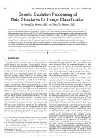
genetic evolution processing of data structures for image classification

Genetic Evolution Processing of
Data Structures for Image Classification
Siu-Yeung Cho, Member, IEEE, and Zheru Chi, Member, IEEE
Abstract—This paper describes a method of structural pattern recognition based on a genetic evolution processing of data structures
with neural networks representation. Conventionally, one of the most popular learning formulations of data structure processing is
Backpropagation Through Structures (BPTS) [7]. The BPTS algorithm has been successfully applied to a number of learning tasks that
involved structural patterns such as image, shape, and texture classifications. However, this BPTS typed algorithm suffers from the
long-term dependency problem in learning very deep tree structures. In this paper, we propose the genetic evolution for this data
structures processing. The idea of this algorithm is to tune the learning parameters by the genetic evolution with specified chromosome
structures. Also, the fitness evaluation as well as the adaptive crossover and mutation for this structural genetic processing are
investigated in this paper. An application to flowers image classification by a structural representation is provided for the validation of
our method. The obtained results significantly support the capabilities of our proposed approach to classify and recognize flowers in
terms of generalization and noise robustness.
Index Terms—Adaptive processing of data structures, genetic algorithm, image classification, and neural networks.
æ
1INTRODUCTION
I
N many application domains in the field of pattern
recognition and classification, it is more appropriate to
model objects by data structures. The topological behavior
in the structural representation provides significant infor-
mation to describe the nature of objects. Unfortunately,
most connectionist models assume that data are organized
by relatively poor structures, such as arrays or sequences,
rather than by a hierarchical manner. In recent years,
machine learning m odels conceived for dealing with
sequences have been straightforwardly adapted to process
data structures. For instance, in image processing, a basic
issue is how to understand a particular given scene. Fig. 1
shows a tree representation of a flower image that can be
used for content-based flower image retrieval and flower

classification. Obviously, the image can be segmented into
two major regions (i.e., the background and foreground
regions) and flower regions can then be extracted from the
foreground region. A tree-structure representation (to some
extent of a semantic representation) can then be established
and the image content can be better described. The leaf
nodes of the tree actually represent individual flower
regions and the root node represents the whole image.
The intermediate tree nodes denote combined flower
regions. For flower classification, such a representation will
take into account both flower regions and the background.
All the flower regions and the background in the tree
representation will contribute to the flower classification to
different extents partially decided by the tree structure. The
tree-structure processing by these specified models can
carry out on the sequential representation based upon the
construction of trees. However, this approach has two
major drawbacks. First, the sequential mapping of data
structures, which are necessary to break some regularities
inherently associated with the data structures, hence they
will yield poor generalization. Second, since the number of
nodes grows exponentially with the depth of the trees, a
large number of parameters need to be learned, which
makes learning difficult and inefficient.
Neural networks (NNs) for adaptive processing of data
struc tures are of paramount importance for stru ctural
pattern recognition and classification [1]. The main motiva-
tion of this adaptive processing is that neural networks are
able to classify static information or temporal sequences
and to perform automatic inferring or learning [2], [3].

Sperduti and Starita proposed supervised neural networks
for the classification of data structures [4]. This approach is
based on using generalized recursive neurons [1], [5]. Most
recently, some advances in this area have been presented
and some preliminary results have been obtained [6], [7],
[8]. The basic idea of a learning algorithm for this
processing is to extend a Backpropagation Through Time
(BPTT) algorithm [9] to encode data structures by recursive
neurons. The so-called recursive neurons means that a copy
of the same neural network is used to encode every node of
the tree structure. In the BPTT algorithm, the gradients of
the weights to be updated can be computed by back-
propagating the error through the time sequence. Similarly,
if learning is performed on a data structure such as a
directed acyclic graph (DAG ), the gradients can be
computed by backpropagating the error through the data
structures, which is known as the Backpropagation
Through Structure (BPTS) algorithm [5]. However, this
gradient-based learning algorithm has several shortcom-
ings. First, the rate of convergence is slow so that the
learning process cannot guarantee completing within a
reasonable time for most complex problems. Although the
algorithm can be accelerated simply by using a larger
learning rate, this would probably introduce oscillation and
might result in a failure in finding an optimal solution.
216 IEEE TRANSACTIONS ON KNOWLEDGE AND DATA ENGINEERING, VOL. 17, NO. 2, FEBRUARY 2005
. S Y. Cho is with the Division of Computing Systems, School of Computer
Engineering, Nanyang Technological University, 50 Nanyang Ave.,
Singapore 639798. E-mail:
. Z. Chi is with the Department of Electronic and Information Engineering,

The Hong Kong Polytechnic University, Hung Hom, Kowloon, Hong
Kong. E-mail:
Manuscript received 1 July 2003; revised 1 Jan. 2004; accepted 19 Apr. 2004;
published online 17 Dec. 2004.
For information on obtaining reprints of this article, please send e-mail to:
, and reference IEEECS Log Number TKDE-0109-0703.
1041-4347/05/$20.00 ß 2005 IEEE Published by the IEEE Computer Society
Second, gradient-based algorithms are usually prone to
local minima [10]. From a theoretical point of view, we
believe that gradient-based learning is not very reliable for
rather complex error surfaces formulated in the data
structure processing. Third, it is extremely difficult for the
gradient-based BPTS algorithm to learn a very deep tree
structure because of the problem of long-term dependency
[11], [12]. Indeed, the gradient contribution disappears at a
certain tree level when the error backpropagates through a
deep tree structure (i.e., the learning information is latched).
This is because the decreasing gradient terms tend to be
zero since the backpropagating error is recursively multi-
plied by the derivative (between 0 and 1) of the Sigmoid
function in each neural node. This results in convergence
stalling and yields a poor generalization.
In view of the rather complex error surfaces formulated by
the adaptive processing of data structures, we need more
sophisticated learning schemes to replace the gradient-based
algorithm so as to avoid the learning being converged to a
suboptimal solution. In our study, a Genetic-based Neural
Network Processing of Data Structures (GNNPoDS) is
developed to solve the problems of long-term dependency
and local minima. Genetic Algorithm (GA) or Evolutionary

Computing (EC) [13], [14], [15] is a computational model
inspired by population genetics. It has been used mainly as
function optimizers and it has been demonstrated to be
effective in the global optimization. Also, GA has been
successfully applied to many multi objective optimizations.
Genetic evolution learning for NNs [16], [17] has been
introduced to perform a global exploration of the search
space, thus avoiding t he problem of stagnation that is
characteristic of local search procedures. There are a number
of different ways for GA implementation as the choice of
genetic operations can be taken in various combinations.
During evolving the parameters of o ur proposed NN
processing, the usual approach is to code the NN as a string
obtained by concatenating the parameter values in one after
another. The structure of the strings corresponds to para-
meters to be learned and may vary depending on how we
impose a certain fitness criteria. In our study, two string
structures are proposed. The first one is called “whole-in-
one” structure. Each parameter represents in12-bits code and
all parameters are arranged into a long string. Simple fitness
criteria based on the error between the target and the output
values can be applied to this kind of string structure, but the
problem lies in the slow convergence because the dimension
of the strings is large. As the string is not a simple chain like
DNA structure, rather it is in a multidimensional form,
performing crossover would become a rather complicated
issue. A simple single point crossover is not applicable for
this structure; rather, a window crossover is suitable to be
performed where a fixed window size of crossover segments
is optimized. The second string structure is called

“4-parallel” structure. Each parameter in four groups is
represented in 12-bit code and all parameters are arranged
into four parametric matrices, each of which is dealt with
independently in the neural network processing of data
structures. It is a much faster approach compared with the
“whole-in-one” structure, but a correlation among different
groups of parameters to be learned may not be imposed
directly for fitness evaluation based only on the error
between the target and output values. Therefore, introducing
appropriate fitness function is an important issue. Among
many different kinds of encoding schemes available, the
binary encoding isapplied because of its simplicity. Mutation
and crossover size (i.e., window size in the “whole-in-one”
structure) are determined and adjusted according to the best
fitness among the population, which results in improving the
GA convergence. Our proposed GA-based NN processing of
data structures are evaluated by flower images classifications
[18]. In this application, semantic image contents are
represented by a tree-structure representation in which the
algorithm can characterize the image features at multilevels
to be beneficial to image classification by using a small
number of simple features. Experimental results illustrate
that our proposed algorithm enhances the learning perfor-
mance significantly in terms of quality of solution and the
avoidance of the long-term dependency problem in the
adaptive processing of data structures.
This paper is organized as follows: The basic idea of the
neural network processing of data structures is presented in
Section 2. A discussion on the problem of long-t erm
dependency for this processing is also given in this section.

Section 3 presents the genetic evolution of the proposed
neural network processing. Section 4 describes the method
of generating the flower image representation by means of
the tree structure and illustrates the working principle of
this proposed application. Section 5 gives the simulation
results and discussion of our study. Finally, a conclusion is
drawn in Section 6.
2NEURAL NETWORK PROCESSING OF DATA
STRUCTURES (NNPODS)
In this paper, the problem of devising neural network
architectures and learning algorithms for the adaptive
processing of data structure is addressed in the content of
classification of structured patterns. The encoding method
CHO AND CHI: GENETIC EVOLUTION PROCESSING OF DATA STRUCTURES FOR IMAGE CLASSIFICATION 217
Fig. 1. A tree representation of a flower image.
by recursive neural networks is based on and modified by
the research works of [1], [4]. We consider that a structured
domain D and all graphs (the tree is a special case of the
graph). In the following discussion, we will use either graph
or tree when it is appropriate. G is a learning set
representing the task of the adaptive processing of data
structures. This representation by the recursive neural
network is shown in Fig. 2.
As shown in Fig. 2, a copy of the same neural network
(shown on the right-side of Fig. 2b) is used to encode every
node in the graph G. Such an encoding scheme is flexible
enough to allow the model to deal with DAGs of different
internal structures and with a different number of nodes.
Moreover, the model can also naturally integrate structural
information into its processing. In the Directed Acyclic

Graph (DAG) shown in Fig. 2a, the operation is run forward
for each graph, i.e., from terminals nodes (N3 and N4) to the
root node (N1). The maximum number of children for a
node (i.e., the maximum branch factor c) is predefined for a
task domain. For instance, a binary tree (each node has two
children only) has a maximum branch factor c equal to two.
At the terminal nodes, there will be no inputs from children.
Therefore, the terminal nodes are known as frontier nodes.
The forward recall is in the direction from the frontier nodes
to the root in a bottom-up fashion. The bottom-up
processing from a child node to its parent node can be
denoted by an operator q
À1
. Suppose that a maximum
branch factor of c has been predefined, each of the form q
À1
i
,
i ¼ 1; 2 ; :c, denotes the input from the ith child node into
the current node. This operator is similar to the shift
operator used in the time series representation. Thus, the
recursive network for the structural processing is formed as
x ¼ F
n
Aq
À1
y þ Bu
ÀÁ
; ð1Þ
y ¼ F

p
Cx þ DuðÞ; ð2Þ
where x, u, and y are the n-dimensional output vector of the
n hidden layer neurons, the m-dimensional inputs to the
neurons, and the p-dimensional outputs of the neurons
respectively. q
À1
is a notation indicating that the input to the
node is taken from its child so that,
q
À1
y ¼
q
À1
1
y
q
À1
2
y
.
.
.
q
À1
c
y
0
B
B

B
@
1
C
C
C
A
: ð3Þ
The parametric matrix A is defined as follows:
A ¼
A
1
A
2
ÁÁÁ A
c
ÀÁ
; ð4Þ
where c denotes the maximum number of children in the
graph. A is an n Á c Á pðÞmatrix such that each A
k
, k ¼
1; 2; ;c is an n Á p matrix, which is formed by the vectors
a
i
j
, j ¼ 1; 2; ;n. B, C, and D are, respectively, n Á mðÞ,
p Á nðÞ, and p Á mðÞ-dimensional matrices. F
n
ÁðÞand F

p
ÁðÞare
n and p-dimensional parametric vectors, respectively, given
as follows:
F
n
ðÞ¼
f
1
ðÞ
f
2
ðÞ
.
.
.
f
n
ðÞ
0
B
B
B
@
1
C
C
C
A
; ð5Þ

where fðÞis the nonlinear function defined as
fðÞ¼1= 1 þ e
À
ðÞ:
2.1 BackPropagation through Structure (BPTS)
Algorithm
In accordance with the research work by Hammer and
Sperschnedier [19], based on the theory of the universal
approximation of the recursive neural network, a single
hidden layer is sufficient to approximate any complicated
mapping problems. The input-output learning task can be
defined by estimating the parameters A, B, C, and D in the
parame terization from a set of training (in put-output)
examples. Each input-output example can be formed in a
tree data structure consisting of a number of nodes with
their inputs and target outputs. Each node’s inputs are
described by a set of attributes u. The target output is
denoted by t, where t is a p-dimensional vector. So, the cost
function is defined as a total sum-squared-error function:
218 IEEE TRANSACTIONS ON KNOWLEDGE AND DATA ENGINEERING, VOL. 17, NO. 2, FEBRUARY 2005
Fig. 2. An illustration of a data structure with its nodes encoded by a single-hidden-layer neural network. (a) A Directed Acyclic Graph (DAG) and
(b) the encoded DAG.
J ¼
1
2
X
N
T
i¼1
t

i
À y
R
i
ÀÁ
T
t
i
À y
R
i
ÀÁ
; ð6Þ
where N
T
is the total number of the learning data
structures. y
R
denotes the output at the root node. Note
that in the case of structural learning processing, it is often
assumed that the attributes, u, are available at each node of
the tree. The main step in the learning algorithm involves
the following gradient learning step:
kþ 1ðÞ¼kðÞÀ
@J
@





¼ðkÞ
; ð7Þ
where kðÞdenotes the free learning parameters  :
A; B; C; D
fg
at the kth iteration and  is a learning rate.
@J
@


¼ðkÞ
is the partial derivative of the cost function with
respect to  evaluated at  ¼ kðÞ. The derivation of the
learning algorithm involves the evaluation of the partial
derivative of the cost function with respect to the
parameters in each node. Thus, the general form of the
derivatives of the cost function with respect to the
parameters is given by:
@J
@
¼À
X
N
T
i¼1
t À y
R
i
ÀÁ
T

à y
R
i
ÀÁ
 r

x
i
ðÞ; ð8Þ
where à yðÞis a p Á p diagonal matrix defined by the first
derivative of the nonlinear activation function.  is defined
as n-dimensional vector which is the fu nction of the
derivative of x with respect to the parameters. It can be
evaluated as:
r

x ¼ Ã xðÞAq
À1
@y
@
; ð9Þ
where à xðÞis a n Á n diagonal matrix defined in a similar
manner as à yðÞ. It is noted that q
À1
@y
@
essentially repeats the
same computation such that the evaluation depends on the
structure of the tree. This is called either the folding
architecture algorithm [5] or backpropagation through

structure algorithm [4].
In the formulation of the learning structural processing
task, it is not required to assume a priori knowledge of any
data structures or any a priori information concerning the
internal structures. Howeve r, we need to assume the
maximum number of children for each node in the tree is
predefined. The parameterization of the structural proces-
sing problem is said to be an overparameterization if the
predefined maximum number of children is so much
greater than that of real trees, i.e., there are many
redundancy parameters in the recursive network than
required to describe the behavior of the tree. The over-
parameterization may give rise to the problem of local
minima in the BPTS learning algorithm. Moreover, the long-
term dependency problem may also affect the learning
performance of the BPTS approach due to the vanishing
gradient information in learning deep trees. The learning
information may disappear at a certain level of the tree
before it reaches at the frontier nodes so that the conver-
gence of the BPTS stalls and a poor generalization results. A
detailed analysis of this problem will be given in the next
section.
2.2 Long-Term Dependency Problem
For backpropagation learning of multilayer perceptron
(MLP) networks, it is well-known that if there are too many
hidden layers, the parameters at very deep layers are not
updated. This is because backpropagating errors are multi-
plied by the derivative of the sigmoidal function, which is
between 0 and 1 and, hence, the gradient for very deep
layers could become very small. Bengio et al. [11] and

Hochreiter and Schmidhuber [20] have analytically ex-
plained why backprop learning problems with the long-
term depen dency a re difficult. They stated that the
recurrent MLP network is able to robustly store information
for an application of long temporal sequences when the
states of the network stay within the vicinity of a hyperbolic
attractor, i.e., the eigenvalues of the Jacobian are within the
unit circle. However, Bengio et al. have shown that if its
eigenvalues are inside the unit circle, then the Jacobian at
each time step is an exponentially decreasing function. This
implies that the portion of gradients becomes insignificant.
This behavior is called the effect of vanishing gradient or
forgetting behavior [11]. In this section, we briefly describe
some of the key aspects of the long-term dependency
problem learning in the processing of data structures. The
gradient-based learning algorithm updates a set of para-
meters  : A; B; C; D
fg
in the recursive neural network for
node representation defined in (1) and (2) such that the
updated parameter can be denoted as
Á ¼ r

J; ð10Þ
where  is a learning rate and r

is the matrix defined as
r

¼

@
@
1
@
@
2
ÁÁÁ
@
@
n
hi
: ð11Þ
By using the chain rule, the gradient can be expressed as:
r

J ¼À
X
N
T
i¼1
t
i
À y
R
i
ÀÁ
T
r
x
R

y
R
i
r

x
R
: ð12Þ
If we assume that computing the partial gradient with
respect to the parameters of the node representation at
different levels of a tree is independent, the total gradient is
then equal to the sum of these partial gradients as:
r

J ¼À
X
N
T
i¼1
t
i
À y
R
i
ÀÁ
T
r
x
R
y

R
i
Á
X
R
l¼1
J
R;RÀl
x
r

l
x
l
!
; ð13Þ
where l ¼ 1 R represents the levels of a tree and J
R;RÀl
x
¼
r
x
l x
R
denotes the Jacobian of (1) expanded over a tree from
level R (root node) to l backwardly. Based on the idea of
Bengio et al. [11], the Jacobian J
R;n
x
is an exponentially

decreasing function of n since the backpropagating error is
multiplied by the derivative of the Sigmoidal function
which is between 0 and 1, so that lim
n!1
J
R;n
x
¼ 0. This
implies that the portion of r

J at the bottom levels of trees
is insignificant compared to the portion at the upper levels
of trees. The effect of vanishing gradients is the main reason
why the BPTS algorithm is not sufficiently reliable for
discovering the relationships between desired outputs and
inputs, which we term the problem of long-term depen-
dency. Therefore, we are now proposing a genetic evolution
method to avoid this effect of vanishing gradients by the
BPTS algorithm so that the evaluation for updating the
parameters becomes more robust in the problem of deep
tree structures.
CHO AND CHI: GENETIC EVOLUTION PROCESSING OF DATA STRUCTURES FOR IMAGE CLASSIFICATION 219
3GENETIC EVOLUTION FOR PROCESSING OF DATA
STRUCTURES
The genetic evolution neural network introduces an
adaptive and global approach to learning, especially in
the reinforcement learning and recurrent neural network
learning paradigm where gradient-based learning often
experiences great difficulties on finding the optimal solu-
tion [16], [17]. This section presents using the genetic

algorithm for evolving neural network processing of data
structures. In our study, the major objective is to determine
the parameters  : A; B; C; D
fg
of the recursive neural
network in (1) and (2) over the whole data structures. Our
proposed genetic approach consists of two major considera-
tions. The first one is to consider the string representation of
the parameters, i.e., either in form of “whole-in-one”or
“4-parallel” structure. These two string representations will
be discussed in the next section. Based on these two
different string structures, the objection function for fitness
criterion is the other main consideration. Different string
representations and object functions can lead to quite
different learning performance. A typical cycle of the
evolution of learning parameters is shown in Fig. 3. The
evolution terminates when the fitness is greater than a
predefined value (i.e., the objective function reaches the
stopping criterion) or the population has converged.
3.1 String Structure Representation
The genetic algorithm always uses binary strings to encode
alternative solutions, often termed chromosomes. In such a
representation scheme, each parameter is represented by a
number of bits with certain length. The recursive neural
network is encoded by concatenation of all the parameters
in the chromosome. Basically, the merits of the binary
representation lie in its simplicity and generality. It is
straightforward to apply the classical crossover (such as the
single-point or multipoint crosso ver) and mutation to
binary strings. There are several encoding methods (such

as uniform, gray, or exponential) that can be used in the
binary representation. The gray code is suggested to
alleviate the Hamming distance problem in our study. It
ensures that the codes for adjacent integers always have a
Hamming distance of one so that the Hamming distance
does not monotonously increase with the difference in
integer values. In the string structure representation, a
proper string structure for GA operations is selected
depending on fitness evaluation. One of a simple way is a
“whole-in-one” structure in which all parameters are
encoded into one long string.
The encoding for the “whole-in-one” structure is simple
and the objective function is simply evaluated by the error
between the target and the root output values of data
220 IEEE TRANSACTIONS ON KNOWLEDGE AND DATA ENGINEERING, VOL. 17, NO. 2, FEBRUARY 2005
Fig. 3. The genetic evolution cycle for the neural network processing of data structure.
structures. But, the dimension may be very high so that the
GA operations may be inefficient. Moreover, this “whole-in-
one” structure representation has the permutation problem.
It is caused by the many-to-one mapping from the
chromosome representation to the recursive neural network
since two different networks have an equivalent function
but they have different chromosomes. This permutation
problem makes the crossover operator very inefficient and
ineffective in producing good offspring. Thus, another
string structure representation called “4-parallel” structure
is used to overcome the above problem. The GA process
becomes efficient when we apply it over each group of
parameters individually. It is likely to perform a separate
GA process on each group of parameters in parallel, but the

limitation lies on its inability of performing the correlation
constrains among the learning parameters of each node. The
objective function is essentially designed for this “4-parallel”
string structure so as to evaluate the fitness criteria for GA
operations of structural processing. In (1) and (2), the
recursive network for the structure processing is rewritten
in matrices form as
xh
1
h
2
y

¼ F
AB
CD

Á
q
À1
yx
uu
&'
: ð14Þ
Note that h
1
and h
2
are used as two dummy vectors. The
matrix

AB
CD

can be encoded into one binary string for the “whole-in-one”
structure. A very long chromosome is formed as:
chromosomeðA; B; C; DÞ :¼
00100 . . . 0000110
fgj
d¼nÁðcÁpÞþnÁmþpÁnþpÁm
:
ð15Þ
On the other hand, for the “4-parallel” structure representa-
tion, four binary strings in the dimensions of n Á c Á pðÞ, n Á m,
p Á n, and p Á m, respectively, for the parametric matrices A,
B, C, and D are formed as
chromosomeðAÞ :¼ 00100 . . . 0000110fgj
d¼nÁðcÁpÞ
; ð16aÞ
chromosomeðBÞ :¼ 00100 . . . 0000110fgj
d¼nÁm
; ð16bÞ
chromosomeðCÞ :¼ 00100 . . . 0000110
fgj
d¼pÁn
; ð16cÞ
chromosomeðDÞ :¼ 00100 . . . 0000110fgj
d¼pÁm
: ð16dÞ
Note that d represents the number of parameters to be
learned so that the total size of this chromosome is d Á

number of encoding bits.
3.2 Objective Function for Fitness Evaluation
The genetic algorithm with the arithmetic crossover and
nonuniform mutation is employed to optimize the para-
meters in the neural processing of data structures. The
objective function is defined as a mean-squared-error
between the desired output and the network output at the
root node:
E
a
¼
P
N
T
i¼1
t
i
À y
R
i
ÀÁ
T
t
i
À y
R
i
ÀÁ
N
T

Á p
; ð17Þ
where N
T
is the total number of the data structures in the
learning set. t and y
R
denote p-dimensional vectors of the
desired output and the real output at the root node. For
GA operations, the objective is to maximize the fitness value
by setting the chromosome to find the optimal solution. In
order to perform operations in the “whole-in-one” structure
representation, the fitness evaluation can be simply defined
based on E
a
fitness
a
¼
1
1 þ
ffiffiffiffiffiffi
E
a
p
: ð18Þ
Basically, the above fitness is applied to the “whole-in-one”
structure but cannot be applied directly to the “4-parallel”
string structure. The objective function for the “4-parallel”
string representation is evaluated as follows: Let an error
function, e

i
ðÞ¼t
i
À y
i
jj
, be approximated by a first-order
Taylor series as,
e
i
ðÞ%e
i

0
ðÞþr

e
i
Á Á; ð19Þ
where  ¼ A; B; C; D
fg
represents the parameters of our
proposed processing and, so,
r

¼À
@
@A
@
@B

@
@C
@
@D
ÈÉ
: ð20Þ
Therefore, (19) becomes:
e
i
ðÞ%
e
i

0
ðÞþÀ
@y
i
@A
Á ÁA À
@y
i
@B
Á ÁB À
@y
i
@C
Á ÁC À
@y
i
@D

Á ÁD

:
ð21Þ
In (21), the first term is the initial error term while the
second term can be denoted as a smoothness constraint that
is given by the output derivatives of learning parameters.
Thus, the objective function of this constraint becomes,
E
b
¼
P
N
T
i¼1
À
@y
R
i
@
Á Á

N
T
: ð22Þ
So, the fitness evaluation for the “4-parallel” string structure
representation is thus determined:
fitness
b
¼

1
1 þ 
ffiffiffiffiffiffi
E
a
p
þ 1 À ðÞE
b
; 0  1; ð23Þ
where  is a constant and ð1 ÀÞ weights the smoothness
constraint. It is noted that the range of the above fitness
evaluation is within [0,1]. This smoothness constraint is a
trade off between the ability of the GA convergence and the
correlation among four groups of parameters. In our study,
we empirically set  ¼ 0:9.
3.3 Selection Process
Chromosomes in the popu lation are selected for the
generation of new chromosomes by a selection scheme. It
is expected that a better chromosome will generate a larger
number of offsprings, and has a higher chance of surviving
in the subsequent generation. The well-known Roulette
CHO AND CHI: GENETIC EVOLUTION PROCESSING OF DATA STRUCTURES FOR IMAGE CLASSIFICATION 221
Wheel Selection [21] is used as the selection mechanism.
Each chromosome in the population is associated with a
sector in a virtual wheel. According to the fitness value of
the chromosome, which is proportional to the area of the
sector, the chromosome that has a higher fitness value will
occupy a larger sector while a lower value takes the slot of a
smaller sector. The selection rate of chromosome (s), is
determined by:

rate sðÞ¼
F À fitness sðÞ
P
size
À 1ðÞÁF
; ð24Þ
where F is the sum of the fitness values of all chromosomes
and P
size
is the size of chromosome population. In our
study, the selection rate is predefined such that the
chromosome is selected if the rate is equal to or smaller
than the predefined rate. In our study, the predefined rate is
set as 0.6.
Another selection criterion of the chromosome may be
considered on the constant  in the fitness function (23)
which takes the form as follows: Assume that at least one
chromosome has been successfully generated in the
population P , i.e., 9s
i
2 P , such that E
a
s
i
ðÞ!0, then the
fitness evaluation becomes:
fitness s
i
ðÞ¼
1

1 þ 1 À ðÞE
b
s
i
ðÞ
: ð25Þ
Consider that chromosome s
j
2 P fail to be chosen in
learning, i.e., E
a
s
j
ÀÁ
> 0 )
ffiffiffiffiffiffiffiffiffiffiffiffiffiffi
E
a
ðs
j
Þ
p
>> E
b
s
j
ÀÁ
, so:
fitness s
j

ÀÁ
¼
1
1 þ 
ffiffiffiffiffiffiffiffiffiffiffiffiffiffi
E
a
ðs
j
Þ
p
: ð26Þ
Hence,  is selected as follows to ensure
fitness s
j
ÀÁ
< fitness s
i
ðÞ;
then

ffiffiffiffiffiffiffiffiffiffiffiffiffiffi
E
a
ðs
j
Þ
q
> 1 À ðÞE
b

s
i
ðÞ; ð27Þ
so
>
E
b
s
i
ðÞ
ffiffiffiffiffiffiffiffiffiffiffiffiffiffi
E
a
ðs
j
Þ
p
þ E
b
s
i
ðÞ
: ð28Þ
As our empirical study defines the constant value of
 ¼ 0:9, the chromosome is successfully selected by satisfy-
ing the criter ion in (28). To sum up, suppose that a
chromosome, s
test
, will be selected if it satisfies the
following conditions:

if
F À fitness s
test
ðÞ
P
size
À 1ðÞÁF
0:6 and
E
b
s
test
ðÞ
ffiffiffiffiffiffiffiffiffiffiffiffiffiffiffiffiffiffi
E
a
ðs
test
Þ
p
þ E
b
s
test
ðÞ
< 0:9:
3.4 Crossover and Mutation Operations
There are se veral ways to implement the crossover
operation depending on the chromosome structure. The
single point crossover is appropriate for the “4-parallel”

structure, but it is not applicable for the “whole-in-one”
structure because of its high dimension. It is more
appropriate to implement the window crossover for the
“whole-in-one” encoding, where the crossover point and
the size of the window are taken within a valid range.
Basically, the point crossover operation with the probability
rate p
ca
is applied in the “whole-in-one” chromosome. Once
the probability test has passed (i.e., a random number is
smaller than p
ca
), the crossover point is determined.
Besides, the crossover window size is determined by the
best fitness (fitness
best
) among the chromosome population.
The idea is that the window size is forced to decrease as the
square of the best fitness value increases. So, the window
size is:
W
size
¼ N
bit
À N
crossover
ðÞ
Á 1 À fitness
2
best

ÀÁ
; ð29Þ
where N
bit
denotes the number of bits in the “whole-in-one”
chromosome and N
crossover
denotes the crossover point in
the chromosome. The crossover operation of this “whole-in-
one” structure is illustrated in Fig. 4. The parents are
separated into two portions by a randomly defined cross-
over point and the size of the portions is determined by (29).
The new chromosome is then formed by combining the
shading portions of two parents as indicated in Fig. 4.
For another chromosome structure as “4-parallel” struc-
ture since the size of this structure is smaller than that of the
“whole-in-one” structure, single-point crossover operation
can thus be applied directly. There are four crossover rates
to be assigned with the four groups of parameters, so that if
a random number is smaller than the probability, the new
chromosome is mated from the first portion of the parent 1
and the last portion in the parent 2. The crossover operation
for this “4-parallel” structure is shown in Fig. 5.
Mutation introduces variations of the model parameters
into chromosomes. It provides a global searching capability
for the GA by randomly altering the values of string in the
chromosomes. Bit mutation is applied for the above two
chromosome structures in the form of bit-string. This is a
random operation that occasionally (with probability p
mb

,
typically between 0.01 and 0.05) occurs which alters the
value of a string bit so as to introduce variations into the
chromosome. A bit is flipped if a probability test is satisfied.
4STRUCTURE-BASED FLOWER IMAGE
CLASSIFICATION
Flower classification is a very challenging problem and will
find a wide range of applications including live plant
resource and data management, and education on flower
taxonomy [18]. There are 250,000 named species of flower-
ing plants and many plant species have not been classified
and named. In fact, flower classification or plant identifica-
tion is a very demanding and time-consuming task, which
has mainly been carried out by taxonomists/botanists. A
significant improvement can be expected if the flower
classification can be carried out by a machine-learning
model with the aid of image processing and computer
vision techniques. Machine learning-based flower classifi-
cation from color images is and will continue to be one of
the most difficult tasks in computer vision due to the lack of
proper models or representations, the large number of
biological variations that a species of flowers can take, and
imprecise or ambiguous image preprocessing results. Also,
there are still many problems in accurately locating flower
regions when the background is complex. It is due to its
complex structure and the nature of 3D objects which adds
another dimension of difficulty in modeling. Flowers can,
basically, be characterized by color, shape, and texture.
Color is a main feature that can be used to differentiate
flowe rs from the background includi ng le aves, stems,

shadows, soils, etc. Color-based domain knowledge can be
222 IEEE TRANSACTIONS ON KNOWLEDGE AND DATA ENGINEERING, VOL. 17, NO. 2, FEBRUARY 2005
adopted to delete pixels that do not belong to flower
regions. Das et al. [27] proposed an iterative segmentation
algorithm with a knowledge-driven mechanism to extract
flower regions from the background. Van der Heijden and
Vossepoel proposed a general contour-oriented shape
dissimilarity measure for a comparison of flowers of potato
species [28]. In another study, a feature extraction and
learning approach was developed by Saitoh and Kaneko for
recognizing 16 wild flowers [29]. Four flower features
together with two leaf features were used as the input for
training the neural network flower classifier. A quite good
performance was achieved by their holistic approach.
However, the approach can only handle single flower
orientation to classify the corresponding category. It cannot
be directly extended to several different flower orientations
with the same species (i.e., they are the same species but in
different orientations and colors).
Image c ontent representation has b een a popular
research topic in various images processing applications
for the past few years. Most of the approaches represent the
image content using only low-level visual features either
globally or locally. It is noted that high-level features (such
as Fourier descriptors or wavelet domain d escrip tors)
cannot characterize the image contents accurately by their
spatial relationships whereas local features (such as color,
shape, or spatial texture) depend on error-prone segmenta-
tion results. In this study, we consider a region-based
representation cal led binary tree [22], [23], [24]. The

construction of ima ge representation is based on t he
extraction of the relevant regions in the image. This is
typically obtained by a region-based segmentation in which
the algorithm can extract the interesting regions of flower
images based on a color clustering technique in order to
simulate human visual perception [30]. Once the regions of
CHO AND CHI: GENETIC EVOLUTION PROCESSING OF DATA STRUCTURES FOR IMAGE CLASSIFICATION 223
Fig. 4. Window crossover operation for the “whole-in-one” structure.
Fig. 5. Parallel crossover operation for the “4-parallel” string structure.
interest have been extracted, a node is added to the graph
for each of these regions. Relevant regions to describe the
objects can be merged together based on a merging strategy.
Binary trees can be formed as a semantic representation
whose nodes correspond to the regions of the flower image
and arcs represent the relationships among regions. Beside
the extraction of the structure, a vector of real value
attributes is compute d to describe the image regions
associated by the node. The features include color informa-
tion, shading/contrast properties, and invariant shape
characteristics. The following sections describe how to
construct the binary trees representation for flower images.
Fig. 6 illustrates the system architecture of the structure-
based flower images classification. At the learning phase, a
set of binary tree patterns representing flower images under
different families were generated by the combining pro-
cesses of segmentation, mergi ng strategy, and feature
extraction. All these tree patterns were used for training
the model by our proposed genetic evolution processing in
data structures. At the classification phase, a query image is
supposed to be classified automatically by the trained

neural network in which the binary tree was generated by
the same processes for generating learning examples.
4.1 Segmentation
A color image is usually given by R (red), G (green), and B
(blue) values at every pixel. But, the difficulty with the RGB
color model is that it produces color components that do not
closely follow those of the human visual system. A better
color model produces color components that follow the
understanding of color by H (hue), S (saturation), and I
(intensity or luminance) [25]. Of these three components,
the hue is considered as a key component in the human
perception. However, the HSI color model has several
limitations. First, the model gives equal weighting to the
RGB components when computing the intensity or lumi-
nance of an image. This does not correspond with the
brightness of a color as perceived by the eye. The second
one is that the length of the maximum saturation vector
varies depending on the hue of the color. Therefore, from
the color clustering point of view, it is desired that the
image is represented by color features which constitute a
space pos sessing unifor m character istics such as the
ðL
Ã
;a
Ã
;b
Ã
Þ color channels system [26]. It was shown that
this system gives good results in segmenting the color
images. The values of the ðL

Ã
;a
Ã
;b
Ã
Þ are obtained by
transforming the (R, G, B) values into the (X, Y, Z) space
which is further converted to a cube-root system. The
transformation is shown below:
X
Y
Z
2
4
3
5
¼
2:7690 1:7518 1:1300
1:0000 4:5907 0:0601
0:0000 0:0565 5:5943
2
4
3
5
Á
R
G
B
2
4

3
5
; ð30aÞ
L
Ã
¼ 116
Y
Y
0

1
3
À16; with
Y
Y
0
> 0:01; ð30bÞ
a
Ã
¼ 500
X
X
0

1
3
À
Y
Y
0


1
3
()
; with
X
X
0
> 0:01; ð30cÞ
b
Ã
¼ 200
Y
Y
0

1
3
À
Z
Z
0

1
3
()
; with
Z
Z
0

> 0:01; ð30dÞ
where X
0
, Y
0
, and Z
0
are the (X, Y, Z) values of the reference
white color (i.e., 255 for the 8-bit gray-scale image). Thus,
the cube-root system yields a simpler decision surface in
accordance with human color perception. They are given by
lightness : L
Ã
; ð31aÞ
224 IEEE TRANSACTIONS ON KNOWLEDGE AND DATA ENGINEERING, VOL. 17, NO. 2, FEBRUARY 2005
Fig. 6. System architecture of the flower classification.
hue : H

¼ tan
À1
b
Ã
a
Ã

; ð31bÞ
chroma : C
Ã
¼
ffiffiffiffiffiffiffiffiffiffiffiffiffiffiffiffiffiffiffiffiffiffiffiffiffiffiffiffiffiffiffiffi

ða
Ã
Þ
2
þðb
Ã
Þ
2

r
: ð31cÞ
The proposed segmentation uses the Euclidean distance
to measure the similarity between the selected cluster and
the image pixels within the above cube-root system. The
first step of our method is to convert the RGB components
into the lightness-hue-chroma channel based on (30) and
(31). The Euclidean distance between each cluster centroid
and the image pixels within the lightness-hue-chroma
channel is given as:
D
i
¼
ffiffiffiffiffiffiffiffiffiffiffiffiffiffiffiffiffiffiffiffiffiffiffiffiffiffiffiffiffiffiffiffiffiffiffiffiffiffiffiffiffiffiffiffiffiffiffiffiffiffiffiffiffiffiffiffiffiffiffiffiffiffiffiffiffiffiffiffiffiffiffiffiffiffiffiffiffiffiffiffiffiffiffiffiffiffiffiffiffiffiffiffiffiffiffiffiffiffiffiffiffiffiffiffiffiffiffiffiffiffiffi
L
Ã
x; yðÞÀL
Ã
i
ÀÁ
2

þ H

x; yðÞÀH

i
ÀÁ
2
þ C
Ã
x; yðÞÀC
Ã
i
ÀÁ
2
q
;
for 1 i M;
ð32Þ
where M is the number of selected clusters. L
Ã
i
;H

i
;C
Ã
i
ÀÁ
is
the ith cluster centroid and ðL

Ã
ðx; yÞ;H

ðx; yÞ;C
Ã
ðx; yÞÞ is
the image pixel at the coordinates x and y within the cube-
root system. For clustering the regions of interest, the k-
mean clustering method [25] is used such that a pixel ðx; yÞ
is identified as belonging to background cluster j if
min
i2
D
i
x; yðÞ
fg
¼ D
j
. For the above computation, the
determination of the cluster centroids is very crucial. They
can be evaluated by:
L
Ã
i
¼
1
N
i
X
L

Ã
x;yðÞ2
i
L
Ã
x; yðÞ; ð33aÞ
H

i
¼
1
N
i
X
H

x;yðÞ2
i
H

x; yðÞ; ð33bÞ
C
Ã
i
¼
1
N
i
X
C

Ã
x;yðÞ2
i
C
Ã
x; yðÞ; ð33cÞ
where N
i
is the number of pixels assigned to cluster 
i
. The
number of assigned clusters is based on the number of the
most dominant peaks determining by the k-mean clustering
within the chroma channel. For example, Fig. 7 illustrates a
flower image with a histogram of the chroma channel in
which there are two most dominant peaks within the
channel (i.e., clusters “a” and “b”). Thus, two clusters can be
assigned. One of them should be the background cluster
whereas another should be the foreground cluster. The
segmentation results of this example image are shown in
Fig. 8 in which two images (Figs. 8a and 8b) are segmented
with two cluster centroids and the corresponding flower
region is extracted as shown in Fig. 8c.
4.2 Merging Strategy and Tree Construction
The idea of creating and processing a tree-structure image
representation is an attempt t o take benefit from the
attractive features of the segmentation results based on
the method described in the previous section. In our study,
we start from the terminated nodes and merge two similar
neighboring regions associated with the child nodes based

on their contents. This merging is iteratively operated by a
recursive algorithm until the child nodes of the root node
(i.e., the background and foreground regions). The follow-
ing explains the proposed merging strategy to create a
binary tree. Assume that the merged regions pair is denoted
as OR
i
;R
j
ÀÁ


i6¼j
2 
i;j
, where R
i
;R
j
for i; j ¼ 1 P denote
the P regions and the entropy function is M
R
i
[R
j
for a pair
of regions R
i
and R
j

for the merging criterion. The merging
criterion is based on examining the entropy of all pairs of
regions to identify which one is the maximum and the
merging is terminated until the last pair of regions merged
to become the entire image. At each step, the algorithm
searches for the pair of most similar regions’ contents,
which should be the pair of child nodes linked with their
parent node. The most similar regions pair is determined by
maximizing the entropy:
OR
i
;R
j
ÀÁ


i6¼j
¼ arg max
OR
i
;R
j
ðÞ
2
i;j
M
R
i
[R
j



i6¼j
no
: ð34Þ
The entropy function M
R
i
[R
j
of regions R
i
and R
j
is
computed based on the color homogeneity of two sub-
regions, which is defined as:
M
R
i
[R
j


i6¼j
¼À
N
R
i
N

T
X
K
k¼1
p
R
i
k
log
2
p
R
i
k
þ
N
R
j
N
T
X
K
k¼1
p
R
j
k
log
2
p

R
j
k
!
;
ð35Þ
where N
R
i
;N
R
j
are the number of pixels for two regions R
i
and R
j
, N
T
is the total number of pixels for the parent
region, K is the number of quantized c olors, and p
k
represents the percentages of the pixels at the kth color in
CHO AND CHI: GENETIC EVOLUTION PROCESSING OF DATA STRUCTURES FOR IMAGE CLASSIFICATION 225
Fig. 7. (a) A single flower image example and (b) its histogram of Chroma channel.
the region. The above computation is done recursively until
no more regions can be merged. For a flower image as
shown in Fig. 9a, the image is segmented into four regions,
so the algorithm merges them in three steps. In the first
step, suppose that the pair of most similar regions is regions
“a” and “b,” which can be merged to create “e.” Then, node

“e” is merged with region “c” to create “f” corresponding to
the foreground region. Finally, node “f” is merged with
region “d” corresponding to the background region to
create “g” which is the root node corresponding to the
whole image. The merging sequence is:
e ¼ Oa;bðÞ!f ¼ Oc;eðÞ!g ¼ Od;fðÞ;
and the tree constructed is shown in Fig. 9b. The merging
order is based on the color homogeneity criterion as well
as the number of merged regions. Fig. 10 shows the tree
construction results of the other two examples from our
flower images database. Such a region-based binary tree
representation considers the foreground flower regions as
well as the background containing leaves and tree
branches. The representation takes into consideration the
contribution and distribution of multiple flowers. There-
fore, the representation is more meaningful than using a
single flower region or combined flower regions in a flat-
vector representation. We believe that this is a necessary
step eventually leading to a more robust semantic image
content representation.
4.3 Feature Extraction
Besides the creation of the tree structure-based image
representation, the features of each region must be
computed and attached to the corresponding node in the
tree. The features can be visual features, such as color,
texture, and shape, which are very important in character-
izing image contents. In the tree structural representation,
the content of a region can be well characterized by the
features including color, shape, and statistical texture
attributes. Four attributes describing color, two simple

statistical texture features, and four attributes of shape are
extracted to characterize a region (a node in the binary tree).
All these 10 attributes are extracted and attached to each
node of the tree. Color attributes include the percentage of
the number of quantized colors in the region over that in the
whole image and the percentages of the three most
dominant colors in the RGB color space. For each of 8-bits
R, G, and B components, we consider two most significant
bits. Therefore, the total possible numbers of color levels are
64 bins ð4 Á 4 Á 4Þ. These four attributes are very useful for
characterizing the color property of a region. For extracting
the texture features from an image region, we present the
textures of a region in terms of two statistical attributes (i.e.,
mean and standard deviation) to characterize the texture.
Apart from the color and texture features, shape features
are desirable in characterizing various flower regions. In
fact, it is rather difficult to extract shape descriptors which
are insensitive to large variations in image scale, rotation,
and translation. In our study, two features are used to
describe the shape of a flower region. Two attributes are
used to describe the edge densities in both vertical and
horizontal directio ns of the flower region. The edge
densities can be evaluated by finding the area in the
histograms of edge informationinbothverticaland
horizontal directions. Also, the position of a flower region
has no effect on the edge directions. We also present
another shape feature of a flower region in terms of second-
order invariant moments (two attributes). These features
are invariant under rotation, scale, translation, and reflec-
tion of the image. In total, four attributes are used to

represent the shape features. Using a small number of
simple features to describe each image region is actually the
other main merit of our tree structural representation of
flowers.
5EXPERIMENTAL RESULTS AND DISCUSSION
This section reports the performance of the flower image
classification by the genetic evolution processing of data
226 IEEE TRANSACTIONS ON KNOWLEDGE AND DATA ENGINEERING, VOL. 17, NO. 2, FEBRUARY 2005
Fig. 8. The segmentation results of a flower image example. (a) Segmentation by cluster centriod “a” in the histogram shown in Fig. 7b.
(b) Segmentation by cluster centriod “b” in the histogram shown in Fig. 7b. (c) The extracted flower region by the segmentation result with the
selected cluster centriod “b.”
Fig. 9. Example of region merging to create a binary tree. (a) Four
regions (including the background region) created by the segmentation
and (b) four-levels binary tree.
structures with the structural image representation. The
image classification was performed on eight families of
flowers in which they are classified in terms of their
living features in flowering plant taxonomy. The eight
flower familiess for our experiments are Amaryllidaceae,
Asteraceae, Brassicaceae, Clematis, Rosaceae, Liliaceae,
Malvaceae, and Violaceae. Fig. 11 shows the examples of
these eight families from our flower database. Some
images are with a single flower and some images are
with multiple numbers of flowers. Most of the flower
images were collected by us and some of them were
downloaded from the Internet. The flower database
consists of 933 images from 79 flower species. 575
images were used to generate a learning set for training
and the other 358 images were used for classification. In
our study, each image was represented by three to five

different trees in accordance with different k values
(normally set to 3 to 5) for the k-mean clustering during
the segmentation process. Therefore, about 3,400 tree-
structure patterns were generated in both learning and
testing sets. In our investigations, we compared the
performance of our proposed genetic evolution algorithm
with conventional neural classifiers based on the multi-
layer perceptron (MLP) network and the radial basis
function (RBF) network. We also used the backpropaga-
tion through structure (BPTS) learning algorithm to
compare with our proposed algorithm to exhibit an
ability of overcoming the long-term dependency pro-
blem. The testing was also performed under different
types and conditions of noise. A single-hidden-layer
recursive neural network was used to encode the node
representation of tree structures. As there are 10 input
attributes and eight families for this classification
problem, we set the configuration of 10-8-8. The
parameter (weight) initialization is performed randomly
in the range of [-1, 1] with a uniform distribution.
5.1 Learning Performance Evaluations
In our study, the learning methods to be compared include
the MLP and RBF networks with flat-vector input patterns
either region features-based or node features-based. The
region features based input to the MLP and RBF classifiers
is a vector of 10 input attributes according to the feature
extraction methods in Section 4.3. The features were
extracted from each region generated from the segmenta-
tion method based on the method in Section 4.1. The vector
components for all regions are arranged to form a flat

vector. Another node features based input vector is a long
vector of 10 input attributes (in the same feature extraction
schemes) obtained by arranging the input attributes of each
node from the tree construction according to the method in
Section 4.2. Also, our proposed genetic evolution algorithm
is compared with the BPTS learning for the structural
processing. In this comparative studies, the number of
nodes at the hidden layer is the same among the different
neural classifiers but the number of parameters (weights)
used are different, which are dependent on what features
based input are used (i.e., region-based or node-based from
the tree). For instance, the number of parameters used for
the sequential processing with the flat-vector input is
greater than that of the structural processing. The difference
in the number of hidden nodes reflects t he different
computational complexity of different classifiers. Suppose
that a classifier has m hidden nodes and n input features,
the computational complexity of sequential processing with
the flat-vector input with region-based features, flat-vector
input with node features, and structural processing of
binary tree, are, respectively, Âðr Á n Á mÞ, Âðð2
r
À 1ÞÁn Á mÞ,
and Âðð2c þ nÞÁmÞ, where r and c represent the number of
segmented regions and the number of categories, respec-
tively. Their classification results are tabulated in Table 1.
The comparative results show that our proposed genetic
evolution algorithm exhibits a better performance with an
average classification rate of 86 percent, whereas 60 percent,
65 percent, and 70 percent were obtained, respectively, for

the MLP classifier, the RBF classifier, and the BPTS learning
for processing of data structures.
CHO AND CHI: GENETIC EVOLUTION PROCESSING OF DATA STRUCTURES FOR IMAGE CLASSIFICATION 227
Fig. 10. Examples of tree structures constructed from the two flower images from the same class in the flower database. (a) Single flower in an
image. (b) The segmentation result from (a). (c) The tree constructed based on (b). (d) Three flowers in an image. (e) The segmentation result from
(d). (f) The tree constructed based on (e).
5.2 Noise Robustness
Apart from the above classification results, the noise
sensitivity is another important issue to be evaluated.
Experiments were conducted for patterns corrupted by
different types and conditions of noise. The flower
images were corrupted by three different types of noise,
namely, “Gaussian,” “Salt and Pepper,” and “Multi-
plicative” with noise levels in the range of 0 percent to
10 percent. Noise corrupted patterns were, respectively,
obtained by changing the intensity of each pixel with
certain distributions (i.e., certain degrees of mean and
variance), changing the intensity of each uncorrelated
pixel with a certain probability, and adding a certain
random degree of noise to each pixel based on a random
variable of uniform distribution with a zero mean. The
overall comparative results are tabulated in Table 2. The
classification rates were obtained by averaging 20
228 IEEE TRANSACTIONS ON KNOWLEDGE AND DATA ENGINEERING, VOL. 17, NO. 2, FEBRUARY 2005
Fig. 11. Examples of eight different families of flower images. Families: (a) Amaryllidaceae, (b) Asteraceae, (c) Brassicaceae, (d) Clematis,
(e) Rosaceae, (f) Liliaceae, (g) Malvaceae, and (h) Violaceae.
TABLE 1
A Comparison among Different classifiers with Different Learning Methods in the Classification of Eight Species of Flowers
TABLE 2
Average Classification Rates by Different Classifiers under Different Noise Conditions

independent runs under different initializations and
different noise conditions. In fact, using the MLP and
RBF classifiers with the flat-vector input has broken some
regularities inherently associated with the data structures,
which yield poor generalization, especiall y on the
condition of noise corruption. Moreover, th e neura l
processing of data structures by BPTS learning algorithm
is suffered from the problem of long-term dependency
that has been discussed in the previous section. The
overall classification rate obtained by our proposed
genetic processing of data structure with both the
“whole-in-one” and the “4-parallel” chromosome struc-
tures are around 85 percent without noise and 80 percent
with noise conditions. On the contrary, approximately 70
percent was obtained by the BPTS learning algorithm.
The overall classification rates of the tested methods for
different noise conditions are shown in Figs. 12a, 12b,
and 12c. The results show that the derivation of
classification rates among these methods is smaller under
lower noise level, but they trend to increase as the noise
level increases. The results also illustrate that our
approach is more robust to the noise.
5.3 Classification on an Extended Data Set
To further evaluate how well our system performs for
flower classification, a selection of images corresponding to
the studied flower families were downloaded from the
internet ( to extend our test
flower database. Each image is represented by three binary
trees automatically generated by using a combination of
segmentation, merging strategy, and feature extractions

according to the schemes in Section 4. In this evaluation,
five flower species in each category were selected to be
added and each species has two to three images under
different orientations. Therefore, the number of flower
species was extended to 84 and the total number of testing
images became 459. Although the exact characteristic of
CHO AND CHI: GENETIC EVOLUTION PROCESSING OF DATA STRUCTURES FOR IMAGE CLASSIFICATION 229
Fig. 12. Overall classification rates of different classification methods against different noise levels of (a) “Gaussian” noise, (b) “Salt and Pepper”
noise, and (c) “Multiplicative” noise.
TABLE 3
Classification Confusion Matrix in Extended Testing Data Set
each test image is unknown, the classification performed by
our structure-based classifier can be used to categorize from
the binary tree representation, wh ich is then visuall y
compared to the images database for retrieval. The
classification accuracy is shown by the confusion matrix
in Table 3. The result is encouraging and consistent in the
extension of the testing flower database to classify more
numbers of flower species.
6CONCLUSION
In this paper, we propose a new approach to image
classification, which is referred to as an adaptive
processing of data structures with the genetic evolution
learning. Unlike conventional connectionist and statistical
approaches, which typically rely on a static representation
of data resulting in vectors of features, patterns can be
better represented by directed graphs/trees, which are
subsequently processed using specific neural networks. In
this paper, we emphasize that it is extremely difficult for
the gradient-based Backpropagation Through Structure

(BPTS) algorithm to learn a very deep tree structure
because of the problem of long-term dependency. Indeed,
the gradient contribution disappears at a certain level of
tree structures due to the effect of the vanishing gradient
or the forgetting behavior. In our study, we develop a
genetic evolution processing to overcome this problem. In
this proposed framework, the parameters/weights are
tuned by genetic evolution with adaptive crossover and
mutation. Two different chromosome structures, namely,
“whole-in-one” and “4-parallel,” are proposed. The
“4-parallel” structure delivers slightly better results than
the “whole-in-one” structure under the specific fitness
evaluation. Also, the convergence rate of the “4-parallel”
is faster than that of the “whole-in-one” structure. In this
paper, experimental results on flower image classification
have shown the advantages of our proposed algorithm.
We considered a region-based binary tree representation
to represent the image at multiple levels and the
connect ivity between regions is translation invariant.
Different evaluations, including learning performance
and noise robustness, are also shown that our proposed
approach can produce a promising performance for the
application to flower classification and recognition. Also,
our approach is more robust to noise than the other
methods tested.
ACKNOWLEDGMENTS
The work described in this paper is partially supported by a
grant from the Research Grants Council of the Hong Kong
Special Administrative Region, China (Project No.: PolyU
5119/01E) and an ASD grant from the Hong Kong

Polytechnic University (Project No.: A408).
REFERENCES
[1] C.L. Giles and M. Gori, Adaptive Processing of Sequences and Data
Structures. New York, Springer, 1998.
[2] A.C. Tsoi, “Gradient Based Learning Methods,” Adaptive Proces-
sing of Sequences and Data Structures, C.L. Giles and M. Gori, eds.,
pp. 27-62, New York, Springer, 1998.
[3] B. Hammer, “Learning with Recurrent Neural Networks,” Spring-
er Lecture Notes in Control and Information Sciences 254, Springer-
Verlag, 2000.
[4] A. Sperduti and A. Starita, “Supervised Neural Networks for
Classification of Structures,” IEEE Trans. Neural Networks, vol. 8,
pp. 714-735, 1997.
[5] A.C. Tsoi, “Adaptive Processing of Data Structure: An Expository
Overview and Comments,” technical report, Faculty of Infor-
matics, Univ. of Wollongong, Australia, 1998.
[6] P. Frasconi, M. Gori, and A. Sperduti, “A General Framework for
Adaptive Processing of Data Structures,” IEEE Trans. Neural
Networks, vol. 9, pp. 768-785, 1998.
[7] C. Goller and A. Kuchler, “Learning Task-Dependent Distributed
Representations by Back-Propagation through Structure,” Proc.
IEEE Int’l Conf. Neural Networks, pp. 347-352, 1996.
[8] P. Fr ascon i, M. Gori, A. Kuchler, and A. Sperduti, “From
Sequences to Data Structures: Theory and Applications,” A Field
Guild to Dynamical Recurrent Networks, J. Kolen and S. Kremer,
eds., pp. 351-374, chapter 19, IEEE Press, 2001.
[9] D.E. Rumelhart and J.L. McClelland, Parallel Distributed Processing:
Exploration in the Microstructure of Cognition. MIT Press, 1986.
[10] M. Gori and A. Tesi, “On the Problem of Local Minima in
Backpropagation,” IEEE Trans. Pattern Analysis and Machine

Intelligence, vol. 14, no. 1, pp. 76-86, 1992.
[11] Y. Bengio, P. Simard, and P. Frasconi, “Learning Long-Term
Dependencies with Gradient Descent is Difficult,” IEEE Trans.
Neural Networks, vol. 5, no. 2, pp. 157-166, Mar. 1994.
[12] Y. Bengio and P. Frasconi, “Input-Output HMM’s for Sequence
Processing,” IEEE Trans. Neural Networks, vol. 7, no. 5, pp. 1231-
1249, Sept. 1996.
[13] M. Srinivas, “Genetic Algorithms: A Survey,” Computer, pp. 17-26,
June 1994.
[14] K.F. Man, K.S. Tang, and S. Kwong, Genetic Algorithms, Concepts
and Designs. Springer-Verlag, 1999.
[15] T. Back, U. Hammel, and H P. Schwefel, “Evolutionary Compu-
tations: Comments on the History and Current State,” IEEE Trans.
Evolutionary Computation, vol. 1, no. 1, pp. 3-17, Apr. 1997.
[16] X. Yao, “Evolving Artificial Neural Networks,” Proc. IEEE, vol. 87,
no. 9, pp. 1423-1447, Sept. 1999.
[17] V. Maniezzo, “Genetic Evolution of the Topology and Weight
Distribution of Neural Networks,” IEEE Trans. Neural Networks,
vol. 5, no. 1, pp. 39-53, Jan. 1994.
[18] Z. Chi, “Data Management for Live Plant Identificatio n,”
Mutimedia Information Retrieval and Management, D. Feng,
W.C. Siu, and H. Zhang, eds., Springer-Verlag, to be published.
[19] B. Hammer and V. Sperschneider, “Neural Networks Can
Approximate Mappings on Structured Objects,” Proc. Second Int’l
Conf. Computational Intelligence and Neuroscience (ICCIN ’97), 1997.
[20] S. Hochreiter and J. Schmidhuber, “Long Short-Term Memory,”
Neural Computation, vol. 9, no. 8, pp. 1735-1780, 1997.
[21] J.H. Holland, Adaptation in Natural and Artificial System. Ann
Arbor, Mich.: Univ. of Michigan Press, 1975.
[22] X. Wu, “Image Coding by Adaptive Tree-Structured Segmenta-

tion,” IEEE Trans. Information Theory, vol. 38, no. 6, pp. 1755-1767,
Nov. 1992.
[23] H. Radha, M. Vetterli, and R. Leonardi, “Image Compression
Using Binary Space Partitioning Trees,” IEEE Trans. Image
Processing, vol. 5, no. 12, pp. 1610-1624, Dec. 1996.
[24] P. Salembier and L. Garrido, “Binary Partition Tree as an Efficient
Representation for Image Processing, Segmentation, and Informa-
tion Retrieval,” IEEE Trans. Image Processing, vol. 9, no. 4, pp. 561-
576, Apr. 2000.
[25] A.R. Weeks and G.E. Hague, “Color Segmentation in the HSI
Color Space Using the K-means Algorithm,” Proc. SPIE, vol. 3026,
pp. 143-154, 1997.
[26] M. Celenk, “Colour Image Segmentation by Clustering,” IEE
Proc.—E, vol. 138, no. 5, pp. 368-376, Sept. 1991.
[27] M. Das, R. Manmatha, and E.M. Riseman, “Indexing Flower
Patent Images Using Domain Knowledge,” IEEE Intelligent
Systems, pp. 24-33, Sept./Oct. 1999.
[28] G.W.A.M. van der Heijden and A.M. Vossepoel, “A Landmark-
Based Approach of Shape Dissimilarity,” Proc. Int’l Conf. Pattern
Recognition (ICPR ’96), pp. 120-124, 1996.
[29] T. Saitoh and T. Kaneko, “Automatic Recognition of Wild
Flowers,” Proc. 15th Int’l Conf. Pattern Recognition, vol. 2, pp. 507-
510, 2000.
[30] E. Vicario, Image Description and Retrieval. New York and London:
Plenum Press, 1998.
230 IEEE TRANSACTIONS ON KNOWLEDGE AND DATA ENGINEERING, VOL. 17, NO. 2, FEBRUARY 2005
Siu-Yeung Cho received the BEng (Hon s)
degree from the University of Brighton, United
Kingdom, in 1994 and the PhD degree from the
City University of Hong Kong in August 1999, all

in electronic engineering. He is now an assistant
professor in the School of Computer Engineer-
ing, Nanyang Technological University of Singa-
pore. His research interests include neural
networks, pattern recognition, and 3D computer
vision. He has published more than 30 technical
papers. He is a member of the IEEE.
Zheru Chi received the BEng and MEng
degrees from Zhejiang University in 1982 and
1985, respectively, and the PhD degree from the
University of Sydney in March 1994, all in
electrical engineering. Since February 1995, he
has been with the Hong Kong Polytechnic
University, where he is now an associate
professor in the Department of Electronic and
Information Engineering. Since 1997, he has
served as a session organizer/session chair/
area moderator/program committee member for a number of interna-
tional conferences. Dr. Chi was one of contributors to the Comprehen-
sive Dictionary of Electrical Engineering (CRC Press and IEEE Press,
1999). His research inte rest s incl ude image proc essin g, pat tern
recognition, example-based machine translation, and computational
intelligence. He has coauthored one book and seven book chapters, and
published more than 100 technical papers. He is a member of the IEEE.
. For more information on this or any other computing topic,
please visit our Digital Library at www.computer.org/publications/dlib.
CHO AND CHI: GENETIC EVOLUTION PROCESSING OF DATA STRUCTURES FOR IMAGE CLASSIFICATION 231