Tiêu chuẩn iso 05725 3 1994 scan
Bạn đang xem bản rút gọn của tài liệu. Xem và tải ngay bản đầy đủ của tài liệu tại đây (1.54 MB, 34 trang )
Y
INTERNATIONAL STANDARD I S 0 5725-3~1994
TECHNICAL CORRIGENDUM 1
Published 2001-10-15
INTERNATIONALORGANIZATIONFOR STANDARDIZATION
.
MDK~YHAPO~~HAROPrAHmAum no C T A H W T M ~ M M
ORGANISATIONINTERNATIONALEDE NORMALISATION
Accuracy (trueness and precision) of measurement methods and
results Part 3:
Intermediate measures of the precision of a standard measurement
method
TECHNICAL CORRIGENDUM 1
Exactitude oustesse et fidélité) des résultats et méthodes de mesure Partie 3: Mesures intermédiaires de la fidélité d’une méthode de mesure normalisée
RECTIFICATIF TECHNIQUE 1
Technical Corrigendum 1 to International Standard IS0 5725-3:1994 was prepared by Technical Committee
ISOTTC 69, Applications of statistical methods, Subcommittee SC 6 , Measurement methods and results.
Page 14, 4th and 5th lines below Table B.2
Replace
1
4
“ s $ ) = -(MS2-MSI)”
1
Replace “s& = -(MSI-MSe)”
2
with
“.RI
with .$‘ )
1
4
= -(MSI-MSZ)”.
1
2
= -(MS2 -MSe)”.
Page 17, Table C.2, column “Sum of squares” for ”Source O”
ICs 03.120.30
O
Ref. No. I S 0 5725-3:1994/Cor.l:200I(E)
Is0 2001 -All rights reserved
--``````,,,,````,,````,,,````-`-`,,`,,`,`,,`---
Printed in Switzerland
COPYRIGHT 2003; International Organization for Standardization
Document provided by IHS Licensee=Shell Services International B.V./5924979112,
User=, 03/09/2003 21:10:16 MST Questions or comments about this message: please
call the Document Policy Management Group at 1-800-451-1584.
I NTERNAT IO NA L
STANDARD
IS0
5725-3
First edition
1994-12-15
Accuracy (trueness and precision) of
measurement methods and results
-
Part 3:
Intermediate measures of the precision of a
standard measurement method
Exactitude (justesse et fidélité) des résultats et méthodes de mesure Partie 3: Mesures intermédiaires de la fidélité d'une méthode de mesure
normalisée
Reference number
I S 0 5725-3:1994(E)
--``````,,,,````,,````,,,````-`-`,,`,,`,`,,`---
COPYRIGHT 2003; International Organization for Standardization
Document provided by IHS Licensee=Shell Services International B.V./5924979112,
User=, 03/09/2003 21:10:16 MST Questions or comments about this message: please
call the Document Policy Management Group at 1-800-451-1584.
4853903 0594558 082
IS0 5725-3:1994(E)
Contents
Page
1
Scope ..............................................................................................
1
2
Normative references .....................................................................
2
3
Definitions
4
General requirement
5
Important factors
.......................................................................
2
6
Statistical model
........................................................................
3
............................................................................
3
....................................................................
3
....................................................................................
4
.................................................................................
6.1
Basic model
6.2
General mean. m
6.3
Term B
6.4
Terms Bo. i+.).
6.5
Error term, e
.................................................................
2
2
etc ...........................................................
4
...........................................................................
5
7
Choice of measurement conditions
..........................................
5
8
Within-laboratory study and analysis of intermediate precision
...................................................................................
measures
6
..................................................................
8.1
Simplest approach
8.2
An alternative method
............................................................
6
8.3
Effect of the measurement conditions on the final quoted
result
.......................................................................................
7
Interlaboratory study and analysis of intermediate precision
measures
...................................................................................
7
.........................................................
7
..................................................................
7
...............................................................
7
.........................................................
8
................................................
9
9
Underlying assumptions
9.2
Simplest approach
9.3
Nested experiments
9.4
Fully-nested experiment
9.5
Staggered-nested experiment
9.6
Allocation of factors in a nested experimental design
--``````,,,,````,,````,,,````-`-`,,`,,`,`,,`---
9.1
6
........... 9
8 I S 0 1994
All rights reserved . Unless otherwise specified. no part of this publication may be reproduced
or utilized in any form or by any means. electronic or mechanical. including photocopying and
microfilm. without permission in writing from the publisher.
international Organization for Standardization
Case Postale 56 CH-121 1 Genève 20 Switzerland
Printed in Switzerland
Il
COPYRIGHT 2003; International Organization for Standardization
Document provided by IHS Licensee=Shell Services International B.V./5924979112,
User=, 03/09/2003 21:10:16 MST Questions or comments about this message: please
call the Document Policy Management Group at 1-800-451-1584.
= 4853903 0594559
0
~~
TL9
IS0 5725-3:1994(E)
IS0
9.7
9.8
Comparison of the nested design with the procedure given in
I S 0 5725-2
..............................................................................
9
Comparison of fully-nested and staggered-nested experimental
designs
...................................................................................
9
Annexes
A
Symbols and abbreviations used in I S 0 5725
B
Analysis of variance for fully-nested experiments
.......................
................. 12
B.l
Three-factor fully-nested experiment
...................................
12
B.2
Four-factor fully-nested experiment
.....................................
13
C
Analysis of variance for staggered-nested experiments
....... 15
C.1
Three-factor staggered-nested experiment
.........................
15
C.2
Four-factor staggered-nested experiment
...........................
16
C.3
Five-factor staggered-nested experiment
............................
17
C.4
Six-factor staggered-nested experiment
..............................
18
Examples of the statistical analysis of intermediate precision
...........................................................................
experiments
19
D
+
D.l
Example 1 .
Obtaining the [time
operator]-different
intermediate precision standard deviation. sicro). within a specific
...........................
19
laboratory at a particular level of the test
D.2
Example 2 .
Obtaining the time-different intermediate precision
standard deviation by interlaboratory experiment
............... 20
E
Bibliography
............................................................................
25
...
--``````,,,,````,,````,,,````-`-`,,`,,`,`,,`---
COPYRIGHT 2003; International Organization for Standardization
10
Document provided by IHS Licensee=Shell Services International B.V./5924979112,
User=, 03/09/2003 21:10:16 MST Questions or comments about this message: please
call the Document Policy Management Group at 1-800-451-1584.
111
4851703 0574560 730
IS0 5725-3:1994(E)
0
IS0
Foreword
I S 0 (the International Organization for Standardization) is a worldwide
federation of national standards bodies (IS0 member bodies). The work
of preparing International Standards is normally carried out through I S 0
technical committees. Each member body interested in a subject for
which a technical committee has been established has the right to be
represented on that committee. International organizations, governmental
and non-governmental, in liaison with ISO, also take part in the work. I S 0
collaborates closely with the International Electrotechnical Commission
(IEC) on all matters of electrotechnical standardization.
Draft International Standards adopted by the technical committees are
circulated to the member bodies for voting. Publication as an International
Standard requires approval by a t least 75 YO of the member bodies casting
a vote.
International Standard I S 0 5725-3 was prepared by Technical Committee
iSO/TC 69, Applications of statistical methods, Subcommittee SC 6,
Measurement methods and results.
IS0 5725 consists of the following parts, under the general title Accuracy
(trueness and precision) of measurement methods and results:
- Part I: General principles and definitions
- Part 2: Basic method for the determination of repeatability and
reproducibility of a standard measurement method
- Part3:
Intermediate measures of the precision of a standard
measurement method
- Part4: Basic methods for the determination of the trueness of a
standard measurement method
- Part 5: Alternative methods for the determination of the precision
--``````,,,,````,,````,,,````-`-`,,`,,`,`,,`---
of a standard measurement method
- Part 6: Use in practice of accuracy values
Parts 1 to 6 of I S 0 5725 together cancel and replace I S 0 5725:1986,
which has been extended to cover trueness (in addition to precision) and
intermediate precision conditions (in addition to repeatability conditions
and reproducibility conditions).
Annexes A, B and C form an integral part of this part of I S 0 5725. Annexes
D and E are for information only.
iv
COPYRIGHT 2003; International Organization for Standardization
Document provided by IHS Licensee=Shell Services International B.V./5924979112,
User=, 03/09/2003 21:10:16 MST Questions or comments about this message: please
call the Document Policy Management Group at 1-800-451-1584.
D 4851903 0 5 9 4 5 b 3 b77
8
IS0
IS0 5725-3:1994(E)
Introduction
0.1 I S 0 5725 uses two terms "trueness" and "precision" to describe
the accuracy of a measurement method. "Trueness" refers to the closeness of agreement between the average value of a large number of test
results and the true or accepted reference value. "Precision" refers to the
closeness of agreement between test results.
0.2
General consideration of these quantities is given in I S 0 5725-1 and
so is not repeated here. It is stressed that I S 0 5725-1 should be read in
conjunction with all other parts of IS0 5725 because the underlying definitions and general principles are given there.
--``````,,,,````,,````,,,````-`-`,,`,,`,`,,`---
0.3 Many different factors (apart from variations between supposedly
identical specimens) may contribute to the variability of results from a
measurement method, including:
a) the operator;
b) the equipment used;
c) the calibration of the equipment;
d) the environment (temperature, humidity, air pollution, etc.);
e) the batch of a reagent;
f)
the time elapsed between measurements.
The variability between measurements performed by different operators
and/or with different equipment will usually be greater than the variability
between measurements carried out within a short interval of time by a
single operator using the same equipment.
0.4 Two conditions of precision, termed repeatability and reproducibility
conditions, have been found necessary and, for many practical cases,
useful for describing the variability of a measurement method. Under repeatability conditions, factors a) to f) in 0.3 are considered constants and
do not contribute to the variability, while under reproducibility conditions
they vary and do contribute to the variability of the test results. Thus repeatability and reproducibility conditions are the two extremes of precision, the first describing the minimum and the second the maximum
variability in results. Intermediate conditions between these two extreme
conditions of precision are also conceivable, when one or more of factors
V
COPYRIGHT 2003; International Organization for Standardization
Document provided by IHS Licensee=Shell Services International B.V./5924979112,
User=, 03/09/2003 21:10:16 MST Questions or comments about this message: please
call the Document Policy Management Group at 1-800-451-1584.
4853903 0594562 503
I S 0 5725-3:1994(E)
8
IS0
a) to f) are allowed to vary, and are used in certain specified circumstances.
Precision is normally expressed in terms of standard deviations.
0.5 This part of I S 0 5725 focuses on intermediate precision measures
of a measurement method. Such measures are called intermediate as
their magnitude lies between the two extreme measures of the precision
of a measurement method: repeatability and reproducibility standard deviations.
To illustrate the need for such intermediate precision measures, consider
the operation of a present-day laboratory connected with a production
plant involving, for example, a three-shift working system where
measurements are made by different operators on different equipment.
Operators and equipment are then some of the factors that contribute to
the variability in the test results. These factors need to be taken into account when assessing the precision of the measurement method.
that aims at developing, standardizing, or controlling a measurement
method within a laboratory. These measures can also be estimated in a
specially designed interlaboratory study, but their interpretation and application then requires caution for reasons explained in 1.3 and 9.1.
0.7 The four factors most likely to influence the precision of a
measurement method are the following.
a) Time: whether the time interval between successive measurements
is short or long.
b) Calibration: whether the same equipment is or is not recalibrated
between successive groups of measurements.
c) Operator: whether the same or different operators carry out the successive measurements.
d) Equipment: whether the same or different equipment (or the same
or different batches of reagents) is used in the measurements.
0.8 It is, therefore, advantageous to introduce the following M-factordifferent intermediate precision conditions (M= 1, 2, 3 or 4) to take account of changes in measurement conditions (time, calibration, operator
and equipment) within a laboratory.
a) M
=
1: only one of the four factors is different;
b) M = 2: two of the four factors are different;
c) M
= 3:
three of the four factors are different;
d) M
= 4:
all four factors are different.
Different intermediate precision conditions lead to different intermediate
precision standard deviations denoted by si( ), where the specific conditions are listed within the parentheses. For example, siIro) is the inter-
vi
COPYRIGHT 2003; International Organization for Standardization
Document provided by IHS Licensee=Shell Services International B.V./5924979112,
User=, 03/09/2003 21:10:16 MST Questions or comments about this message: please
call the Document Policy Management Group at 1-800-451-1584.
--``````,,,,````,,````,,,````-`-`,,`,,`,`,,`---
0.6 The intermediate precision measures defined in this part of
I S 0 5725 are primarily useful when their estimation is part of a procedure
i)B51903 0594563 44T
8
=
I S 0 5725-3:1994(E)
IS0
mediate precision standard deviation with different times
operators (O).
(T) and
0.9 For measurements under intermediate precision conditions, one or
more of the factors listed in 0.7 is or are different. Under repeatability
conditions, those factors are assumed to be constant.
The standard deviation of test results obtained under repeatability conditions is generally less than that obtained under the conditions for intermediate precision conditions. Generally in chemical analysis, the standard
deviation under intermediate precision conditions may be two or three
times as large as that under repeatability conditions. It should not, of
course, exceed the reproducibility standard deviation.
As an example, in the determination of copper in copper ore, a
collaborative experiment among 35 laboratories revealed that the standard
deviation under one-factor-different intermediate precision conditions (operator and equipment the same but time different) was 1,5 times larger
than that under repeatability conditions, both for the electrolytic gravimetry
and Na,S,O,
titration methods.
--``````,,,,````,,````,,,````-`-`,,`,,`,`,,`---
vi i
COPYRIGHT 2003; International Organization for Standardization
Document provided by IHS Licensee=Shell Services International B.V./5924979112,
User=, 03/09/2003 21:10:16 MST Questions or comments about this message: please
call the Document Policy Management Group at 1-800-451-1584.
4 8 5 3 9 0 3 05945b4 3 8 6
INTERNATIONAL STANDARD 8 I S 0
I S 0 5725-3:1994(E)
Accuracy (trueness and precision) of measurement
methods and results Part 3:
Intermediate measures of the precision of a standard
measurement method
1 Scope
--``````,,,,````,,````,,,````-`-`,,`,,`,`,,`---
1.1 This part of I S 0 5725 specifies four intermediate precision measures due to changes in observation
conditions (time, calibration, operator and equipment)
within a laboratory. These intermediate measures can
be established by an experiment within a specific
laboratory or by an interlaboratory experiment.
Furthermore, this part of I S 0 5725
a) discusses the implications of the definitions of intermediate precision measures;
b) presents guidance on the interpretation and application of the estimates of intermediate precision
measures in practical situations;
C)
does not provide any measure of the errors in
estimating intermediate precision measures;
d) does not concern itself with determining the
trueness of the measurement method itself, but
does discuss the connections between trueness
and measurement conditions.
1.2 This part of I S 0 5725 is concerned exclusively
with measurement methods which yield measurements on a continuous scale and give a single value
as the test result, although the single value may be
COPYRIGHT 2003; International Organization for Standardization
the outcome of a calculation from a set of observations.
1.3 The essence of the determination of these intermediate precision measures is that they measure
the ability of the measurement method to repeat test
results under the defined conditions.
1.4 The statistical methods developed in this part
of I S 0 5725 rely on the premise that one can pool
information from "similar" measurement conditions
to obtain more accurate information on the intermediate precision measures. This premise is a
powerful one as long as what is claimed as "similar"
is indeed "similar". But it is very difficult for this
premise to hold when intermediate precision measures are estimated from an interlaboratory study. For
example, controlling the effect of "time" or of "operator" across laboratories in such a way that they are
"similar", so that pooling information from different
laboratories makes sense, is very difficult. Thus, using
results from interlaboratory studies on intermediate
precision measures requires caution. Withinlaboratory studies also rely on this premise, but in
such studies it is more likely to be realistic, because
the control and knowledge of the actual effect of a
factor is then more within reach of the analyst.
1.5 There exist other techniques besides the ones
described in this part of I S 0 5725 to estimate and to
verify intermediate precision measures within a lab-
Document provided by IHS Licensee=Shell Services International B.V./5924979112,
User=, 03/09/2003 21:10:16 MST Questions or comments about this message: please
call the Document Policy Management Group at 1-800-451-1584.
1
4853703 05945b5 212
I S 0 5725-3:1994(E)
Q
IS0
oratory, for example, control charts (see I S 0 5725-6).
This part of I S 0 5725 does not claim to describe the
only approach to the estimation of intermediate precision measures within a specific laboratory.
3 Definitions
This part of I S 0 5725 refers to designs of experiments such as nested designs. Some basic information
is given in annexes B and C. Other references in this area
The symbols used in I S 0 5725 are given in annex A.
NOTE 1
For the purposes of this part of I S 0 5725, the definitions given in I S 0 3534-1 and I S 0 5725-1 apply.
are given in annex E.
2
4 General requirement
Normative references
--``````,,,,````,,````,,,````-`-`,,`,,`,`,,`---
The following standards contain provisions which,
through reference in this text, constitute provisions
of this part of I S 0 5725. At the time of publication, the
editions indicated were valid. All standards are subject
to revision, and parties to agreements based on this
part of I S 0 5725 are encouraged to investigate the
possibility of applying the most recent editions of the
standards indicated below. Members of IEC and I S 0
maintain registers of currently valid International
Standards.
I S 0 3534-1: 1993, Statistics - Vocabulary and symbols - Part 7: Probability and general statistical
terms.
I S 0 5725-1:I 994, Accuracy (trueness and precision)
of measurement methods and results - Part 1:
General principles and definitions.
I S 0 5725-2:1994, Accuracy (trueness and precision)
of measurement methods and results - Part 2: Basic
method for the determination of repeatability and
reproducibility of a standard measurement method.
IS0 Guide 33:1989, Uses of certified reference materials.
I S 0 Guide 35:1989, Certification of reference materials - General and statistical principles.
Table 1
In order that the measurements are made in the same
way, the measurement method shall have been
standardized. All measurements forming part of an
experiment within a specific laboratory or of an interlaboratory experiment shall be carried out according
to that standard.
5
Important factors
5.1 Four factors (time, calibration, operator and
equipment) in the measurement conditions within a
laboratory are considered to make the main contributions to the variability of measurements (see
table 1).
5.2 "Measurements made at the same time" include those conducted in as short a time as feasible
in order to minimize changes in conditions, such as
environmental conditions, which cannot always be
guaranteed constant. "Measurements made a t different times", that is those carried out at long intervals
of time, may include effects due to changes in environmental conditions.
- Four important factors and their states
Measurement conditions within a laboratory
Factor
State 1 (same)
Time
Calibration
Operator
Equipment
2
COPYRIGHT 2003; International Organization for Standardization
State 2 (different)
Measurements made a t the same
time
No calibration between measurements
Same operator
Same equipment without recalibration
Measurements made at different
times
Calibration carried out between
measurements
Different operators
Different equipment
Document provided by IHS Licensee=Shell Services International B.V./5924979112,
User=, 03/09/2003 21:10:16 MST Questions or comments about this message: please
call the Document Policy Management Group at 1-800-451-1584.
4851903 0594566 159
0
I S 0 5725-3:1994(E)
IS0
5.3 "Calibration" does not refer here to any calibration required as an integral part of obtaining a test
result by the measurement method. It refers to the
calibration process that takes place at regular intervals
between groups of measurements within a laboratory.
operator-different intermediate precision standard
deviation, si(o);
+
[time
operator]-different intermediate precision
standard deviation, siF0);
5.4 In some operations, the "operator" may be, in
fact, a team of operators, each of whom performs
some specific part of the procedure. In such a case,
the team should be regarded as the operator, and any
change in membership or in the allotment of duties
within the team should be regarded as providing a
different "operator".
and many others in a similar fashion.
Statistical model
6.1
5.5 "Equipment" is often, in fact, sets of equipment, and any change in any significant component
should be regarded as providing different equipment.
As to what constitutes a significant component,
common sense must prevail. A change of
thermometer would be considered a significant component, but using a slightly different vessel to contain
a water bath would be considered trivial. A change of
a batch of a reagent should be considered a significant
component. It can lead to different "equipment" or to
a recalibration if such a change is followed by calibration.
Basic model
For estimating the accuracy (trueness and precision)
of a measurement method, it is useful to assume that
every test result, y , is the sum of three components:
y=m+B+e
5.7 Under intermediate precision conditions with M
factor(s) different, it is necessary to specify which
factors are a t state 2 of table 1 by means of suffixes,
for example:
- time-different intermediate precision standard deviation, siCr);
- calibration-different intermediate precision standard deviation, si(c);
COPYRIGHT 2003; International Organization for Standardization
. . . (1)
where, for the particular material tested,
m is the general mean (expectation);
B is the laboratory component of bias under re-
peatability conditions;
e
5.6 Under repeatability conditions, all four factors
are a t state 1 of table 1. For intermediate precision
conditions, one or more factors are at state 2 of
table 1, and are specified as "precision conditions
with M factor(s) different", where M is the number
of factors a t state 2. Under reproducibility conditions,
results are obtained by different laboratories, so that
not only are all four factors at state 2 but also there
are additional effects due to the differences between
laboratories in management and maintenance of the
laboratories, general training levels of operators, and
in stability and checking of test results, etc.
--``````,,,,````,,````,,,````-`-`,,`,,`,`,,`---
[time + operator + equipment]-different intermediate precision standard deviation, silrOE);
is the random error occurring in every
measurement under repeatability conditions.
A discussion of each of these components, and of
extensions of this basic model, follows.
6.2
General mean, m
6.2.1 The general mean, m, is the overall mean of
the test results. The value of m obtained in a
collaborative study (see I S 0 5725-2) depends solely
on the "true value" and the measurement method,
and does not depend on the laboratory, equipment,
operator or time by or at which any test result has
been obtained. The general mean of the particular
material measured is called the "level of the test"; for
example, specimens of different purities of a chemical
or different materials (e.g. different types of steel) will
correspond to different levels.
In many situations, the concept of a true value p holds
good, such as the true concentration of a solution
which is being titrated. The level m is not usually equal
to the true value p; the difference (m - p ) is called the
"bias of the measurement method".
Document provided by IHS Licensee=Shell Services International B.V./5924979112,
User=, 03/09/2003 21:10:16 MST Questions or comments about this message: please
call the Document Policy Management Group at 1-800-451-1584.
3
m
4851903 0594567 095
IS0 5725-3:1994(E)
0
. . . (2)
m=p+d
NOTE 2 Discussion of the bias term 6 and a description
of trueness experiments are given in IS0 5725-4.
6.2.2 When examining the difference between test
results obtained by the same measurement method,
the bias of the measurement method may have no
influence and can be ignored, unless it is a function
of the level of the test. When comparing test results
with a value specified in a contract, or a standard
value where the contract or specification refers to the
true value p and not to the level of the test m, or when
comparing test results obtained using different
measurement methods, the bias of the measurement
method must be taken into account.
6.3 Term B
6.3.1 B is a term representing the deviation of a
laboratory, for one or more reasons, from m, irrespective of the random error e occurring in every test
result. Under repeatability conditions in one laboratory, B is considered constant and is called the "laboratory component of bias".
6.3.2 However, when using a measurement method
routinely, it is apparent that embodied within an
overall value for B are a large number of effects which
are due, for example, to changes in the operator, the
equipment used, the calibration of the equipment, and
the environment (temperature, humidity, air pollution,
etc.). The statistical model [equation (111can then be
rewritten in the form:
y = m +Bo
+ B ( , )+ B p ) + ... + e
. . . (3)
or
y
=p
+ 6 + Bo + B(l) + B p ) + ... + e
. . . (4)
where B is composed of contributions from variates
Bo, B(l), B p ) ... and can account for a number of intermediate precision factors.
4
COPYRIGHT 2003; International Organization for Standardization
In practice, the objectives of a study and considerations of the sensitivity of the measurement method
will govern the extent to which this model is used. In
many cases, abbreviated forms will suffice.
6.4 Terms Bo, B(l),B p ) , etc.
6.4.1 Under repeatability conditions, these terms all
remain constant and add to the bias of the test results. Under intermediate precision conditions, Bo is
the fixed effect of the factor(s) that remained the
same (state 1 of table 11, while B(l),B ( z ) ,etc. are the
random effects of the factor(s) which vary (state 2 of
tablel). These no longer contribute to the bias, but
increase the intermediate precision standard deviation
so that it becomes larger than the repeatability standard deviation.
6.4.2 The effects due to differences between operators include personal habits in operating measurement methods (e.g. in reading graduations on scales,
etc.). Some of these differences should be removable
by standardization of the measurement method, particularly in having a clear and accurate description of
the techniques involved. Even though there is a bias
in the test results obtained by an individual operator,
that bias is not always constant (e.g. the magnitude
of the bias will change according to his/her mental
and/or physical conditions on that day) and the bias
cannot be corrected or calibrated exactly. The magnitude of such a bias should be reduced by use of a
clear operation manual and training. Under such circumstances, the effect of changing operators can be
considered to be of a random nature.
6.4.3 The effects due to differences between
equipment include the effects due to different places
of installation, particularly in fluctuations of the indicator, etc. Some of the effects due to differences
between equipment can be corrected by exact calibration. Differences due to systematic causes between equipment should be corrected by calibration,
and such a procedure should be included in the standard method. For example, a change in the batch of
a reagent could be treated that way. An accepted
reference value is needed for this, for which
I S 0 Guide 33 and I S 0 Guide 35 shall be consulted.
The remaining effect due to equipment which has
been calibrated using a reference material is considered a random effect.
--``````,,,,````,,````,,,````-`-`,,`,,`,`,,`---
In some situations, the level of the test is exclusively
defined by the measurement method, and the concept of an independent true value does not apply; for
example, the Vicker's hardness of steel and the
Micum indices of coke belong to this category. However, in general, the bias is denoted by d (6 = O where
no true value exists), then the general mean m is
IS0
Document provided by IHS Licensee=Shell Services International B.V./5924979112,
User=, 03/09/2003 21:10:16 MST Questions or comments about this message: please
call the Document Policy Management Group at 1-800-451-1584.
= 4853903
0
0594568 T23
IS0 5725-3:1994(E)
IS0
6.4.4 The effects due to time may be caused by
environmental differences, such as changes in room
temperature, humidity, etc. Standardization of environmental conditions should be attempted to minimize these effects.
6.4.5 The effect of skill or fatigue of an operator may
be considered to be the interaction of operator and
time. The performance of a set of equipment may be
different at the time of the start of its use and after
using it for many hours: this is an example of interaction of equipment and time. When the population
of operators is small in number and the population of
sets of equipment even smaller, effects caused by
these factors may be evaluated as fixed (not random)
effects.
6.4.6 The procedures given in I S 0 5725-2 are developed assuming that the distribution of laboratory
components of bias is approximately normal, but in
practice they work for most distributions provided that
these distributions are unimodal. The variance of B is
called the "between-laboratory variance", expressed
as
Var(B)
2
= oL
. . . (5)
However, it will also include effects of changes of
operator, equipment, time and environment. From a
precision experiment using different operators,
measurement times, environments, etc., in a nested
design, intermediate precision variances can be calculated. Var@) is considered to be composed of independent contributions of laboratory, operator, day
of experiment, environment, etc.
Var(B) = Var(B,)
+ Var(B(,)) + Var(B(,)) + ...
. . . (6)
The variances are denoted by
6.5 Error term, e
6.5.1 This term represents a random error occurring
in every test result and the procedures given
throughout this part of I S 0 5725 were developed assuming that the distribution of this error variable is
approximately normal, but in practice they work for
most distributions provided that they are unimodal.
6.5.2 Within a single laboratory, its variance is called
the within-laboratory variance and is expressed as
Var(e)
2
. . . (8)
= aW
ah
6.5.3 It may be expected that
will have different
values in different laboratories due to differences such
as in the skills of the operators, but in this part of
I S 0 5725 it is assumed that, for a properly standardized measurement method, such differences between laboratories should be small and that it is
justifiable to establish a common value of withinlaboratory variance for all the laboratories using the
measurement method. This common value, which is
estimated by the mean of the within-laboratory variances, is called the "repeatability variance" and is
designated by
2
-
er = Var(e)
. . . (9)
This mean value is taken over all the laboratories taking part in the accuracy experiment which remain after outliers have been excluded.
7 Choice of measurement conditions
7.1
In applying a measurement method, many
measurement conditions are conceivable within a
laboratory, as follows:
repeatability conditions (four factors constant);
several intermediate precision conditions with one
factor different;
several intermediate precision conditions with two
factors different;
Var(B(,))
= o(2),
2
etc.
. . . (7)
Var(B) is estimated in practical terms as sf and similar
intermediate precision estimates may be obtained
from suitably designed experiments.
several intermediate precision conditions with
three factors different;
intermediate precision conditions with four factors
different.
In the standard for a measurement method, it is not
necessary (or even feasible) to state all possible pre-
--``````,,,,````,,````,,,````-`-`,,`,,`,`,,`---
COPYRIGHT 2003; International Organization for Standardization
Document provided by IHS Licensee=Shell Services International B.V./5924979112,
User=, 03/09/2003 21:10:16 MST Questions or comments about this message: please
call the Document Policy Management Group at 1-800-451-1584.
5
= 4851903 0594569 968 =
I S 0 5725-3:1994(E)
cision measures, although the repeatability standard
deviation should always be specified. As regards intermediate precision measures, common commercial
practice should indicate the conditions normally encountered, and it should be sufficient to specify only
the one suitable intermediate precision measure, together with the detailed stipulation of the specific
measurement conditions associated with it. The
measurement condition factor(s1 to be changed
should be carefully defined; in particular, for timedifferent intermediate precision, a practical mean time
interval between successive measurements should
be specified.
7.2 It is assumed that a standardized measurement
method will be biased as little as possible, and that
the bias inherent in the method itself should have
been dealt with by technical means. This part of
I S 0 5725, therefore, deals only with the bias coming
from the measurement conditions.
7.3 A change in the factors of the measurement
conditions (time, calibration, operator and equipment)
from repeatability conditions (¡.e. from state 1 to 2 of
table 1) will increase the variability of test results.
However, the expectation of the mean of a number
of test results will be less biased than under repeatability conditions. The increase in the standard deviation for the intermediate precision conditions may be
overcome by not relying on a single test result but by
using the mean of several test results as the final
quoted result.
8
IS0
of factor(s1 between each measurement. It is recommended that n should be at least 15. This may not
be satisfactory for the laboratory, and this method of
estimating intermediate precision measures within a
laboratory cannot be regarded as efficient when
compared with other procedures. The analysis is
simple, however, and it can be useful for studying
time-different intermediate precision by making successive measurements on the same sample on successive days, or for studying the effects of calibration
between measurements.
A graph of (yk - 7)versus the measurement number
k, where yk is the kth test result of n replicate test results and j j is the mean of the n replicate test results,
is recommended to identify potential outliers. A more
formal test of outliers consists of the application of
Grubbs' test as given in subclause 7.3.4 of
I S 0 5725-211994.
The estimate of the intermediate precision standard
deviation with M factor(s) different is given by
where symbols denoting the intermediate precision
conditions should appear inside the parentheses.
8.2
An alternative method
8 Within-laboratory study and analysis
of intermediate precision measures
8.2.1 An alternative method considers t groups of
measurements, each comprising n replicate test results. For example, within one laboratory, a set of t
materials could each be measured, then the intermediate precision factor(s) could be altered and the t
materials remeasured, the procedure being repeated
until there are n test results on each of the t materials.
Each group of n test results shall be obtained on one
identical sample (or set of presumed identical samples
in the case of destructive testing), but it is not essential that the materials be identical. It is only required that the t materials all belong to the interval of
test levels within which one value of the intermediate
precision standard deviation with M factor(s) different
can be considered to apply. It is recommended that
the value of t ( n - 1) should be a t least 15.
8.1 Simplest approach
EXAMPLE
The simplest method of estimating an intermediate
precision standard deviation within one laboratory
consists of taking one sample (or, for destructive
testing, one set of presumably identical samples) and
performing a series of n measurements with a change
One operator performs a single measurement on
each of the t materials, then this is repeated by a
second operator, and possibly by a third operator, and
so on, allowing an estimate of si(o) to be calculated.
7.4 Practical considerations in most laboratories,
such as the desired precision (standard deviation) of
the final quoted result and the cost of performing the
measurements, will govern the number of factors and
the choice of the factor(s) whose changes can be
studied in the standardization of the measurement
method.
--``````,,,,````,,````,,,````-`-`,,`,,`,`,,`---
6
COPYRIGHT 2003; International Organization for Standardization
Document provided by IHS Licensee=Shell Services International B.V./5924979112,
User=, 03/09/2003 21:10:16 MST Questions or comments about this message: please
call the Document Policy Management Group at 1-800-451-1584.
W 4853703 0574570 b8T
Q
IS0 5725-3:1994(E)
IS0
8.2.2 A graph of ( y k - $1 versus the material number
j , where yJkis the k td test result on the jth
material and
$ is the average of the n results on thejth material, is
recommended to identify potential outliers. A more
formal test of outliers consists of the application of
Grubbs' test as given in subclause 7.3.4 of
IS0 5725-2:1994 either for each group separately or
for all tn test results combined.
The estimate of the intermediate precision standard
deviation with M factor(s) different, si( ), is then given
bY
For n = 2 (¡.e. two test results on each material), the
formula simplifies to
I
l
8.3 Effect of the measurement conditions on
the final quoted result
8.3.1 The expectation of 7 is different between one
combination and another of time, calibration, operator
and equipment, even when only one of the four factors changes. This is a limitation on the usefulness of
mean values. In chemical analysis or physical testing,
7 is reported as the final quoted result. In trading raw
materials, this final quoted result is often used for
quality evaluation of the raw materials and affects the
price of the product to a considerable extent.
EXAMPLE
In the international trading of coal, the size of the
consignment can often exceed 70 O00 t, and the ash
content is determined finally on a test portion of only
1 g. In a contract stipulating that each difference of
1 % in ash content corresponds to USD 1,5 per tonne
of coal, a difference of 1 mg in the weighing of ash
by a chemical balance corresponds to 0,l % in ash
content, or USD 0,15 per tonne, which for such a
consignment amounts to a difference in proceeds of
USD 10 500 (from 0,l x 1,5 x 70 000).
8.3.2 Consequently, the final quoted result of
chemical analysis or physical testing should be sufficiently precise, highly reliable and, especially, universal and reproducible. A final quoted result which
can be guaranteed only under conditions of a specific
operator, equipment or time may not be good enough
for commercial considerations.
9 Interlaboratory study and analysis of
intermediate precision measures
9.1 Underlying assumptions
Estimation of intermediate measures of precision
from interlaboratory studies relies on the assumption
that the effect of a particular factor is the same across
all laboratories, so that, for example, changing operators in one laboratory has the same effect as changing operators in another laboratory, or that variation
due to time is the same across all laboratories. If this
assumption is violated, then the concept of intermediate measures of precision does not make sense,
nor do the techniques proposed in the subsequent
sections to estimate these intermediate measures of
precision. Careful attention to outliers (not necessarily
deletion of outliers) must be paid as this will help in
detecting departure from the assumptions necessary
to pool information from all laboratories. One powerful
technique to detect potential outliers is to depict the
measurements graphically as a function of the various
levels of the factors or the various laboratories included in the study.
9.2 Simplest approach
If material a t q levels is sent to p laboratories who
each perform measurements on each of the q levels
with a change of intermediate precision factor(s) between each of the n measurements, then the analysis
is by the same method of calculation as explained in
IS0 5725-2, except that an intermediate precision
standard deviation is estimated instead of the repeatability standard deviation.
9.3
Nested experiments
A further way of estimating intermediate precision
measures is to conduct more sophisticated experiments. These can be fully-nested or staggerednested experiments (for definitions of these terms,
see I S 0 3534-3). The advantage of employing a
nested experimental design is that it is possible, a t
one time and in one interlaboratory experiment, to
estimate not only repeatability and reproducibility
standard deviations but also one or more intermediate
precision standard deviations. There are, however,
--``````,,,,````,,````,,,````-`-`,,`,,`,`,,`---
COPYRIGHT 2003; International Organization for Standardization
Document provided by IHS Licensee=Shell Services International B.V./5924979112,
User=, 03/09/2003 21:10:16 MST Questions or comments about this message: please
call the Document Policy Management Group at 1-800-451-1584.
7
4853703 0594571i 5 L b
IS0 5725-3:1994(E)
Q
certain caveats which must be considered. as will be
explained in 9.8.
The subscripts i, j and k suffixed to the data y in
figure 1 a) for the three-factor fully-nested experiment
represent, for example, a laboratory, a day of experiment and a replication under repeatability conditions,
respectively.
9.4 Fully-nested experiment
A schematic layout of the fully-nes sd experir
a particular level of the test is given in figure 1
n
IS0
t
The subscripts i, j , k and 1 suffixed to the data y in
figure 1 b) for the four-factor fully-nested experiment
represent, for example, a laboratory, a day of experiment, an operator and a replication under repeatability
conditions, respectively.
--``````,,,,````,,````,,,````-`-`,,`,,`,`,,`---
By carrying out the three-factor fully-nested experiment collaboratively in several laboratories, one intermediate precision measure can be obtained a t the
same time as the repeatability and reproducibility
standard deviations, ¡.e. u(o),a(,) and u, can be estimated. Likewise the four-factor fully-nested experiment can be used to obtain two intermediate
precision measures, ¡.e. a(o), a(,),a(2) and ur can be
estimated.
Analysis of the results of an n-factor fully-nested experiment is carried out by the statistical technique
”analysis of variance” (ANOVA) separately for each
level of the test, and is described in detail in
annex B.
FACTOR
O (laboratory)
Øl
1
k ---
2 (residual)
Y i/*
YI11
Yi12
Y I22
Yi21
a) Three-factor fully-nested experiment
FACTOR
O (laboratory)
1
i--I
I
I
r
I
l
2
3 (residual) 1 --YiJkl
Y ill1
Y ,112
Y i121
Yi122
Y I211
Y I212
Yi221
b) Four-factor fully-nested experiment
Figure 1
a
- Schematic layouts for three-factor and four-factor fully-nested experiments
COPYRIGHT 2003; International Organization for Standardization
Document provided by IHS Licensee=Shell Services International B.V./5924979112,
User=, 03/09/2003 21:10:16 MST Questions or comments about this message: please
call the Document Policy Management Group at 1-800-451-1584.
Y1222
m
Q
4853903 0594572 4 5 2
m
I S 0 5725-3:1994(E)
IS0
9.5 Staggered-nested experiment
A schematic layout of the staggered-nested experiment at a particular level of the test is given in
figure 2.
FACTOR
j
O (laboratory)
___
1
1
y 'I
YI1
YI2
YI3
YI4
Figure 2 - Schematic layout of a four-factor
staggered-nested experiment
--``````,,,,````,,````,,,````-`-`,,`,,`,`,,`---
The three-factor staggered-nested experiment requires each laboratory i to obtain three test results.
Test results y;, and yi2 shall be obtained under repeatability conditions, and yi3 under intermediate precision conditions with M factor(s) different
( M = 1, 2 or 3). for example under time-different intermediate precision conditions (by obtaining y,, on a
different day from that on which yIl and y,, were obtained).
In a four-factor staggered-nested experiment, yi4 shall
be obtained under intermediate precision conditions
with one more factor different, for example, under
operator]-different intermediate precision
[time
conditions by changing the day and the operator.
+
Again, analysis of the results of an n-factor
staggered-nested experiment is carried out by the
statistical technique "analysis of variance" (ANOVA)
separately for each level of the test, and is described
in detail in annex C.
9.6 Allocation of factors in a nested
experimental design
The allocation of the factors in a nested experimental
design is arranged so that the factors affected most
by systematic effects should be in the highest ranks
(O, 1, ...1, and those affected most by random effects
COPYRIGHT 2003; International Organization for Standardization
should be in the lowest ranks, the lowest factor being
considered as a residual variation. For example, in a
four-factor design such as illustrated in figure 1 b and
figure2, factor O could be the laboratory, factor 1 the
operator, factor 2 the day on which the measurement
is carried out, and factor 3 the replication. This may
not seem important in the case of the fully-nested
experiment due to its symmetry.
9.7 Comparison of the nested design with
the procedure given in I S 0 5725-2
The procedure given in I S 0 5725-2, because the
analysis is carried out separately for each level of the
test (material), is, in fact, a two-factor fully-nested experimental design and produces two standard deviations, the repeatability and reproducibility standard
deviations. Factor O is the laboratory and factor 1 the
replication. If this design were increased by one factor, by having two operators in each laboratory each
obtaining two test results under repeatability conditions, then, in addition to the repeatability and
reproducibility standard deviations, one could determine the operator-different intermediate precision
standard deviation. Alternatively, if each laboratory
used only one operator but repeated the experiment
on another day, the time-different intermediate precision standard deviation would be determined by this
three-factor fully-nested experiment. The addition of
a further factor to the experiment, by each laboratory
having two operators each carrying out two
measurements and the whole experiment being repeated the next day, would allow determination of the
repeatability, reproducibility, operator-different, timeoperator]-different standard
different, and [time
deviations.
+
9.8 Comparison of fully-nested and
staggered-nested experimental designs
'
An n-factor fully-nested experiment requires 2" - test
results from each laboratory, which can be an excessive requirement on the laboratories. This is the
main argument for the staggered-nested experimental
design. This design requires less test results to produce the same number of standard deviations, although the analysis is slightly more complex and there
is a larger uncertainty in the estimates of the standard
deviations due to the smaller number of test results.
Document provided by IHS Licensee=Shell Services International B.V./5924979112,
User=, 03/09/2003 21:10:16 MST Questions or comments about this message: please
call the Document Policy Management Group at 1-800-451-1584.
9
-
IS0 5725-3:1994(E)
4853903 0594573 399
=
Q
IS0
Annex A
(normative)
Symbols and abbreviations used in IS0 5725
k
s=a+bm
A
Factor used to calculate the uncertainty of an estimate
b
Slope in the relationship
s=a+bm
Component in a test result representing the deviation of a laboratory from the general average
(laboratory component of bias)
B
Component of B representing all
factors that do not change in intermediate precision conditions
Components of B representing factors that vary in intermediate Precision conditions
Intercept in the relationship
lg s = c + d I g m
Test statistics
C,
CCr,,,
Mandel's within-laboratory consistency test statistic
LCL Lower control limit (either action limit or warning
limit)
m
General mean of the test property; level
M
Number of factors considered in intermediate
precision conditions
N
Number of iterations
n
Number of test results obtained in one laboratory at one level (¡.e. per cell)
p
Number of laboratories participating in the interlaboratory experiment
P
Probability
4
Number of levels of the test property in the
interlaboratory experiment
r
Repeatability limit
R
Reproducibility limit
RM Reference material
Critical values for statistical tests
CDf
Critical difference for probability P
CRf
Critical range for probability P
d
Slope in the relationship
Ig s = e + d Ig m
s
Estimate of a standard deviation
s^
Predicted standard deviation
T
Total or sum of some expression
t
Number of test objects or groups
e
Component in a test result representing the random error occurring in every test result
UCL Upper control limit (either action limit or warning
limit)
f
Critical range factor
W
Fp(V1, v2)
p-quantile of the F-distribution with
v1 and v2 degrees of freedom
Weighting factor used in calculating a weighted
regression
w
Range of a set of test results
x
Datum used for Grubbs' test
y
Test result
G
Grubbs' test statistic
h
Mandel's between-laboratory consistency test statistic
10
COPYRIGHT 2003; International Organization for Standardization
Document provided by IHS Licensee=Shell Services International B.V./5924979112,
User=, 03/09/2003 21:10:16 MST Questions or comments about this message: please
call the Document Policy Management Group at 1-800-451-1584.
--``````,,,,````,,````,,,````-`-`,,`,,`,`,,`---
Intercept in the relationship
a
4853903 0594574 225
0
IS0 5725-3:1994(E)
IS0
Arithmetic mean of test results
Symbols used as subscripts
i
Grand mean of test results
C
Ca libration-different
C(
Significance level
E
Equipment-different
/I
Type II error probability
i
Identifier for a particular laboratory
y
Ratio of the reproducibility standard deviation to
the repeatability standard deviation (oR/or)
I(
A
Laboratory bias
j
-
A
A
Estimate of A
d
Bias of the measurement method
2
Estimate of d
R
Detectable difference between two laboratory
biases or the biases of two measurement
methods
p
True value or accepted reference value of a test
property
1
Identifier for intermediate measures of
precision; in brackets, identification of
the type of intermediate situation
j
Identifier
for
a
particular level
(IS0 5725-2).
Identifier for a group of tests or for a
factor ( I S 0 5725-3)
k
Identifier for a particular test result in a
laboratory i a t level j
L
Between-laboratory (interlaboratory)
m
Identifier for detectable bias
M
Between-test-sample
v
Number of degrees of freedom
O
Operator-diff erent
e
Detectable ratio between the repeatability standard deviations of method B and method A
P
Probability
True value of a standard deviation
r
Repeatability
o
Component in a test result representing the
variation due to time since last calibration
R
Reproducibility
z
T
Time-diffe rent
W
Within-laboratory (intralaboratory)
1, 2, 3...
For test results, numbering in the order
of obtaining them
4
$(v)
Detectable ratio between the square roots of
the between-laboratory mean squares of
method B and method A
pquantile of the X*-distribution with
of freedom
Y
degrees
( I ) , (2). (3)... For test results, numbering in the order
of increasing magnitude
--``````,,,,````,,````,,,````-`-`,,`,,`,`,,`---
COPYRIGHT 2003; International Organization for Standardization
Document provided by IHS Licensee=Shell Services International B.V./5924979112,
User=, 03/09/2003 21:10:16 MST Questions or comments about this message: please
call the Document Policy Management Group at 1-800-451-1584.
11
D 4851903 0594575 IbI
m
I S 0 5725-3:1994(E)
Annex B
(normative)
Analysis of variance for fully-nested experiments
The analysis of variance described in this annex has to be carried out separately for each level of the test included
in the interlaboratory experiment. For simplicity, a subscript indicating the level of the test has not been suffixed
to the data. It should be noted that the subscript j is used in this part of I S 0 5725 for factor 1 (factor O being the
laboratory), while in the other parts of I S 0 5725 it is used for the level of the test.
I
~
’
The methods described in subclause 7.3 of I S 0 5725-2:1994 should be applied to check the data for consistency
and outliers. With the designs described in this annex, the exact analysis of the data is very complicated when
some of the test results from a laboratory are missing. If it is decided that some of the test results from a laboratory are stragglers or outliers and should be excluded from the analysis, then it is recommended that all the
data from that laboratory (at the level affected) should be excluded from the analysis.
B. 1 Three-factor fully-nested experiment
The data obtained in the experiment are denoted by y#, and the mean values and ranges are as follows:
Yi =
1 -
(Yi1
+ yi2)
where p is the number of laboratories which have participated in the interlaboratory experiment.
The total sum of squares, SST, can be subdivided as
where
Since the degrees of freedom for the sums of squares SSO, SS1 and SSe are p - 1, p and 2p, respectively, the
ANOVA table is composed as shown in table B.1,
--``````,,,,````,,````,,,````-`-`,,`,,`,`,,`---
12
COPYRIGHT 2003; International Organization for Standardization
Document provided by IHS Licensee=Shell Services International B.V./5924979112,
User=, 03/09/2003 21:10:16 MST Questions or comments about this message: please
call the Document Policy Management Group at 1-800-451-1584.
~~
4853903 0594576 O T B
IS0 5725-3:1994(E)
Table B.l
- ANOVA table for a three-factor fully-nested experiment
Sum of
squares
’Ource
Degrees of
freedom
Mean square
O
cso
P-1
MSO = S S O / ( p - 1)
1
ss1
P
MSI
Residual
SSe
2P
Total
SST
4p - 1
=
SSl/p
MSe = S S e l ( 2 p )
The unbiased estimates sfol, sfl) and sf of
MSO, MS1 and MSe as
C T ~ ~ ) ,
Expected mean square
u,’
2
or
+ 207,) + 4u&
2
+ ZU(,)
2
ur
and o:, respectively, can be obtained from the mean squares
2
1
~ ( 0=
)
4 (MSO - MS1)
1 (MSI - MSe)
sf,) =
S,
2
=
MSe
The estimates of the repeatability variance, one-factor-different intermediate precision variance and reproducibility
variance are, respectively, as follows:
n
:s
2
2
S i ( 1 ) = sr
2
SR = sr
2
2
+ S(1)
2
2
+ s ( l ) + s(0)
B.2 Four-factor fully-nested experiment
--``````,,,,````,,````,,,````-`-`,,`,,`,`,,`---
The data obtained in the experiment are denoted by yIJkl, and mean values and ranges are as follows:
RJk =
1
7
(YIJkl + Y 1 j k 2 )
wljk(l)
= lbijkl
- Yuk21
where p is the number of laboratories which have participated in the interlaboratory experiment.
The total sum of squares, SST, can be subdivided as follows:
where
7,Z(3-ri’
SSO =
I
J
k
l
COPYRIGHT 2003; International Organization for Standardization
= 8 x ( 3 ) 2i
Document provided by IHS Licensee=Shell Services International B.V./5924979112,
User=, 03/09/2003 21:10:16 MST Questions or comments about this message: please
call the Document Policy Management Group at 1-800-451-1584.
13
4851903 0594537 T34
I S 0 5725-3:1994(E)
i
j
k
Q
l
IS0
1
--``````,,,,````,,````,,,````-`-`,,`,,`,`,,`---
Since the degrees of freedom for the sums of squares SSO, SS1, SS2 and SSe are p - 1, p , 2p and 4p, respectively,
the ANOVA table is composed as shown in table 6.2.
Table B.2
- ANOVA table for a four-factor fully-nested experiment
Sum of
squares
Source
Degrees of
freedom
Mean square
Expected mean square
sso
ss 1
P-1
P
MSO = SSO/(p - 1)
2
M S I = SSl/p
2
+ 2up)
+ 4u:,) + 80&
u; + 2 4 ) + 44,)
ur
ss2
2P
MS2
=
SS2/(2p)
uf
Residual
SSe
4P
MSe
=
SSel(4p)
2
or
Total
SST
8p - 1
2
2
2
2
2
2
2
+ 20;~)
2
The unbiased estimates s ( ~ ) s(,),
,
q2)and s, of a(o), a(l),a(Z)and or,respectively, can be obtained from the mean
squares MSO, MSI, MS2 and MSe as follows:
'(0)
-1
8 (MSO - MSI)
-
2
1
4
(MS2 - MS1)
s(~=
)
2
1
s ( ~=
)
2
S,
=
(MSI - MSe)
MSe
The estimates of the repeatability variance, one-factor-different intermediate precision variance, two-factors different intermediate precision variance and reproducibility variance are, respectively, as follows:
2
sr
2
2
SI(I)= sr
+ '(2)
2
2
Ji(2) = sr
+ S(2) + S(1)
2
SR
14
2
= sr
2
2
2
2
2
2
+ s(2) + s(l)
+ $(O)
COPYRIGHT 2003; International Organization for Standardization
Document provided by IHS Licensee=Shell Services International B.V./5924979112,
User=, 03/09/2003 21:10:16 MST Questions or comments about this message: please
call the Document Policy Management Group at 1-800-451-1584.
0
IS0
Annex C
(normative)
Analysis of variance for staggered-nested experiments
--``````,,,,````,,````,,,````-`-`,,`,,`,`,,`---
The analysis of variance described in this annex has to be carried out separately for each level of the test included
in the interlaboratory experiment. For simplicity, a subscript indicating the level of the test has not been suffixed
to the data. It should be noted that the subscript j is used in this part of IS0 5725 for the replications within the
laboratory, while in the other parts of I S 0 5725 it is used for the level of the test.
The methods described in subclause 7.3 of I S 0 5725-2:1994 should be applied to check the data for consistency
and outliers. With the designs described in this annex, the exact analysis of the data is very complicated when
some of the test results from a laboratory are missing. If it is decided that some of the test results from a laboratory are stragglers or outliers and should be excluded from the analysis, then it is recommended that all the
data from that laboratory (at the level affected) should be excluded from the analysis.
C. 1 Three-factor staggered-nested experiment
The data obtained in the experiment within laboratory i are denoted by y;] 0‘ = 1, 2, 3), and the mean values and
ranges are as follows:
-
Yi(1) =
1
(Y,l
+Yi4
W i ( i ) = IYii - ~ i 2 l
where p is the number of laboratories which have participated in the interlaboratory experiment.
The total sum of squares, SST, can be subdivided as follows:
where
Since the degrees of freedom for the sums of squares SSO, SS1 and SSe are p - 1 , p and p, respectively, the
ANOVA table is composed as shown in table C.1.
COPYRIGHT 2003; International Organization for Standardization
Document provided by IHS Licensee=Shell Services International B.V./5924979112,
User=, 03/09/2003 21:10:16 MST Questions or comments about this message: please
call the Document Policy Management Group at 1-800-451-1584.
15
4851903 0594579 8 0 7
IS0 5725-3:1994(E)
0
Sum of
squares
--``````,,,,````,,````,,,````-`-`,,`,,`,`,,`---
So"rce
sso/(p - 1 )
ur
1
ss1
P
ss1IP
ur+-u,
Residual
SSe
P
SSelP
2
6,
Total
SST
31, - 1
5 MS1
MSO - 12
3
3 MSe
MS1 - -
2
5 2
P-1
1
s(,) =
2
sso
2
2
Expected mean square
O
The unbiased estimates sfO), sfl) and sr of
MSO, MS1 and MSe as follows:
s ( ~=
)
Mean square
Degrees of
freedom
2
IS0
2
+
2
3~ ( 1 +) 30(0)
4 2
3 0
2
a(l)
and a:,
respectively, can be obtained from the mean squares
1 MSe
+12
4
sr2 = MSe
The estimates of the repeatability variance, one-factor-different intermediate precision variance and reproducibility
variance are, respectively, as follows:
2
sr
2
Si(i)
2
= sr
2
2
SR = sr
C.2
2
+ S(i)
2
2
+ S(1) + S(O)
Four-factor staggered-nested experiment
The data obtained in the experiment within laboratory i are denoted by y¡, (i = 1 , 2 , 3 , 4 ) , and the mean values and
ranges are as follows:
where p is the number of laboratories which have participated in the interlaboratory experiment.
The ANOVA table is composed as shown in table C.2.
16
COPYRIGHT 2003; International Organization for Standardization
Document provided by IHS Licensee=Shell Services International B.V./5924979112,
User=, 03/09/2003 21:10:16 MST Questions or comments about this message: please
call the Document Policy Management Group at 1-800-451-1584.
4851903 0594580 529
8
IS0 5725-3:1994(E)
IS0
Table C.2
- ANOVA table for a four-factor staggered-nested exDeriment
___
Degrees of
freedom
Sum of squares
Source
O
P-1
1
P
2
P
Residual
P
Total
4p- 1
Mean square
Expected mean square
C.3 Five-factor staggered- nested experiment
The data obtained in the experiment within laboratory i are denoted by y;,
and ranges are as follows:
(J’
= 1, 2, 3, 4, 5), and the mean values
--``````,,,,````,,````,,,````-`-`,,`,,`,`,,`---
where p is the number of laboratories which have participated in the interlaboratory experiment.
The ANOVA table is composed as shown in table C.3.
Table C.3
Degrees of
freedom
Sum of squares
Source
O
- ANOVA table for a five-factor staggered-nested experiment
5m,(4))2- 5P6Y
Mean square
Expected mean square
P-1
I
1
4
2
7 cwi(4)
P
3
2
P
2
P
I
2
7 Cwi(3)
I
3
2
3C W I ( 2 )
1
2
1
ewlcli
I
Residual
P
I
Total
c ccv, - 7)’
5p - 1
1 1
COPYRIGHT 2003; International Organization for Standardization
Document provided by IHS Licensee=Shell Services International B.V./5924979112,
User=, 03/09/2003 21:10:16 MST Questions or comments about this message: please
call the Document Policy Management Group at 1-800-451-1584.
17