molecular dynamics simulation of heat transfer and phase change during

1 Copyright © 2001 by ASME
Proceedings of NHTC'01
35th National Heat Transfer Conference
Anaheim, California, June 10-12, 2001
NHTC2001-20070



MOLECULAR DYNAMICS SIMULATION OF HEAT TRANSFER AND PHASE CHANGE DURING
LASER MATERIAL INTERACTION



Xinwei Wang, Xianfan Xu
*


School of Mechanical Engineering
Purdue University
West Lafayette, IN 47907





* To whom correspondence should be addressed
ABSTRACT
In this work, heat transfer and phase change of an argon
crystal illuminated with a picosecond pulsed laser are
investigated using molecular dynamics simulations. The result
reveals no clear interface when phase change occurs, but a

transition region where the crystal structure and the liquid
structure co-exist between the solid and the liquid. Superheating
is observed during the melting process. The solid-liquid and
liquid-vapor interfaces are found to move with a velocity of
hundreds of meters per second. In addition, the vapor is found
to be ejected from the surface with a velocity close to a
thousand meters per second.

Keywords: heat transfer, phase change, MD simulation, laser-
material interaction, ablation threshold
NOMENCLATURE
F
force
I
laser intensity
k

thermal conductivity
B
k Boltzmann's constant
m
atomic mass
M
P

probability for atoms moving with a velocity v
q
′′
heat flux applied to the surface of the target for thermal
conductivity calculation

r
atomic position
c
r cut off distance
s
r the nearest neighbor distance
t
time
T
t
preset time constant in velocity scaling
t
δ
time step
T
temperature
T
δ
initial temperature increase for calculating the specific
heat
T
∆
final temperature increase for calculating the specific
heat
v
velocity
x
coordinate in x direction
y
coordinate in y direction

z
coordinate in z direction

Greek Symbols

χ
velocity scaling factor
ε
LJ well depth parameter
φ
potential
σ
equilibrium separation parameter
ξ
current kinetic temperature in velocity scaling

Subscripts

i
atomic index

Superscripts

* no-dimensionalized

I. INTRODUCTION
In recent years, ultrashort pulsed lasers have been rapidly
developed and used in materials processing. Due to the
extremely short pulse duration, many difficulties exist in
experimental investigation of laser material interaction such as

measuring the transient surface temperature, the velocity of the
solid-liquid interface, and the material ablation rate. Ultrashort
laser material interaction involves several coupled, non-linear,
and non-equilibrium processes inducing an extremely high
2 Copyright © 2001 by ASME
heating rate (10
16
K/s) and a high temperature gradient (10
11

K/m). The continuum approach of solving the heat transfer
problem becomes questionable under these extreme situations.
On the other hand, the molecular dynamics (MD) simulation,
which solves the movement of atoms or molecules directly, is
suitable for investigating the ultrashort laser material interaction
process. One aim of this work is to use the MD simulation to
investigate heat transfer occurring in ultrashort laser-material
interaction and to compare the results with those obtained with
the continuum approach.
A large amount of work has been dedicated to studying
laser material interaction using MD simulations. Due to the
limitation of computer resources, most work was restricted to
systems with a small number of atoms, thus only qualitative
results such as the structural change due to heating were
obtained. For instance, using quantum MD simulations,
Shibahara and Kotake studied the interaction between metallic
atoms and the laser beam in a system consisting of 13 atoms or
less [1, 2]. Their work was focused on the structural change of
metallic atoms due to laser beam absorption. Häkkinen and
Landman [3] studied dynamics of superheating, melting, and

annealing at the Cu surface induced by laser beam irradiation
using the two-step heat transfer model developed by Anisimov
[4]. This model describes the laser metal interaction in two
steps including photon energy absorption in electrons and
lattice heating through interaction with electrons. A large body
of the MD simulation of laser material interaction was to study
the laser induced ablation in various systems. Kotake and
Kuroki [5] studied laser ablation of a small dielectric system
consisting of 4851 atoms. Laser beam absorption was simulated
by exciting the potential energy of atoms. Applying the same
laser beam absorption approach, Herrmann and Campbell [6]
investigated laser ablation of a silicon crystal containing
approximately 23000 atoms. Zhigileit et al. [7, 8] studied laser
induced ablation of organic solid using the breathing sphere
model, which simulated laser irradiation by vibrational
excitation of molecules. However, because of the arbitrary
properties chosen in the calculation, their calculation results
were qualitative, and were restricted to small systems with tens
of thousands of atoms. Ohmura et al. [9] attempted to study
laser metal interaction with the MD simulation using the Morse
potential function for metals [10]. The Morse potential function
simplified the potential calculation among the lattice and
enabled them to study a larger system with 160,000 atoms. Heat
conduction by the electron gas, which dominated heat transfer
in metal, could not be predicted by the Morse potential
function. Alternatively, heat conduction was simulated using the
finite difference method based on the thermal conductivity of
metal. Laser material interaction in a large system was recently
investigated by Etcheverry and Mesaros [11]. In their work, a
crystal argon solid containing about half a million atoms was

simulated. For laser induced acoustic waves, a good agreement
between the MD simulation and the standard thermoelastic
calculation was observed.
In this work, MD simulations are conducted to study laser
argon interaction. The system under study has 486,000 atoms,
which is large enough to suppress statistical uncertainty. Laser
heating of argon with different laser fluences is investigated.
Laser induced heat transfer, melting, evaporation, material
ablation are emphasized in this work. Phase change relevant
parameters, such as the velocity of solid-liquid and liquid-vapor
interfaces, ablation rate, and ablation threshold fluence are
reported. In section II, theories for the MD simulation used in
this work are introduced. Calculation results are summarized in
section III.

II. THEORY OF MD SIMULATION
Molecular dynamics simulation is a computational method
to investigate the behavior of materials by simulating the atomic
motion controlled by a given potential. Argon is
overwhelmingly explored in MD simulation due to the
meaningful physical constants of the widely-accepted Lennard-
Jones 12-6 (LJ) potential and the less computation time
required than more complicated potentials involving multi-body
interaction or electric static force. In this calculation, an argon
crystal at 50 K is assumed to be illuminated with a spatially
uniform laser beam. The melting and the boiling temperatures
of argon at one atm are 83.8 K and 87.3 K, respectively, while
its critical temperature is 150.87 K. The basic problem involves
solving Newtonian equations for each atom interacting with its
neighbors by means of a pairwise Lennard-Jones force:

∑
=
≠ij
ij
i
i
F
dt
rd
m
2
2
(1)

where
i
m and
i
r are the mass and position of atom i,
respectively,
ij
F is the interaction force between atoms i and j,
which is obtained from the Lennard-Jones potential as
ijijij
rF
∂∂φ
/−= . The Lennard-Jones potential
ij
φ

is written as

















−








=
612
4

ijij
ij
rr
σσ
εφ
(2a)

where
ε
is the LJ well depth parameter,
σ
is the equilibrium
separation parameter, and
ijij
rrr −= . Therefore, the force
ij
F
can be expressed as

ij
ijij
ij
r
rr
F ⋅









+−=
8
6
14
12
6124
σσ
ε
(2b)

A standard method for solving ordinary differential
equations (1) and (2) is the finite difference approach. The
general idea is to obtain the atomic positions, velocities, etc. at
time tt
δ
+ based on the positions, velocities, and other
3 Copyright © 2001 by ASME
dynamic information at time t. The equations are solved on a
step-by-step basis, and the time interval t
δ
is dependent
somehow on the method applied. However, t
δ
is usually much
smaller than the typical time taken for an atom to travel its own
length. Many different algorithms have been developed to solve
Eqs. (1) and (2), of which the Verlet algorithm is widely used

due to its numerical stability, convenience, and simplicity [12].
In this calculation, the velocity Verlet algorithm is used, which
is expressed as:

tttvtrttr
ii
δδδ
)2/()()( ++=+ (3a)

ij
ij
ij
r
tt
ttF
∂
δ∂φ
δ
)(
)(
+
−=+
(3b)

t
m
ttF
ttvttv
i
ij

δ
δ
δδ
)(
)2/()2/3(
+
++=+
(3c)

In the calculation, most time is spent on calculating forces
using Eq. (3b). When two atoms are far away enough from each
other, the force between them is negligible. The distance
between atoms beyond which the interaction force is neglected
is called cutoff distance (potential cutoff),
c
r . In this work,
c
r is
taken as 2.5
σ
, which is a cutoff potential widely used in MD
simulations using the LJ potential. At this distance, the potential
is only about 1.6% of the well depth. In the calculation, the
distance between atoms is first compared with
c
r , and only
when the distance is less than
c
r , the force is calculated. The
comparison of the atomic distance with

c
r is organized by
means of the cell structure and the linked list methods [12]. In
these methods, the computation domain is divided into many
structural cells with a characteristic size of
c
r . To speed up the
calculation, direct evaluation of the force using Eqs. (2) is
avoided by looking up a pre-prepared table for the force in the
range of
2
ij
r from 0.25
2
σ
to
2
c
r , with an interval of 10
-6
2
σ
.
Laser energy absorption in the material is simulated by
scaling the velocities of all atoms in each structural cell by an
appropriate factor. The amount of energy deposited in each cell
is calculated assuming the laser beam is exponentially absorbed
in the target. In order to prevent undesired amplification of
atomic macromotion, the average velocity of atoms in each
layer of structural cells is subtracted before velocity scaling.

Non-dimensionalized parameters are used, which are listed
in Table 1. With non-dimensionalization, Eqs. (1) and (2)
become

∑
=
≠ij
ij
i
F
td
rd
*
2*
*2
)(
(4a)

6*12*
*
)(
1
)(
1
ijij
ij
rr
−=
φ
(4b)

*
8*14*
*
)(
6
)(
12
ij
ijij
ij
r
rr
F ⋅








+−=
(4c)

The form of Eqs. (3a) and (3b) is preserved, while Eq. (3c)
becomes

**********
)()2/()2/3( tttFttvttv

ij
δδδδ
+++=+ (5)

Table 1. Nondimensionalized parameters
Quantity Equation
Time
)4//(
*
εσ
mtt =
Length
σ
/
*
rr =
Mass
1/
*
== mmm
Velocity
mvv /4/
*
ε
=
Potential
εφφ
4/
*
=

Force
)/4/(
*
σε
ijij
FF =
Temperature
ε
4/
*
TkT
B
=

Parameters used in the calculation are listed in Table 2. A
face-centered cubic (fcc) structure is used to initialize atomic
positions. The initial atomic velocities are specified randomly
from a Gaussian distribution based on the temperature.

III. CALCULATION RESULTS
The target studied consists of 90 fcc unit cells in x and y
directions, and 15 fcc unit cells in the z direction. Each unit cell
contains 4 atoms, and the system consists of 486,000 atoms. In
both x and y directions, the computational domain has a size of
48.73 nm. In the z direction, the size of the computation domain
is 17.14 nm with the bottom of the target located at 4.51 nm and
the top surface (laser irradiated surface ) at 12.63 nm.
4 Copyright © 2001 by ASME
Table 2. Values of the parameters used in the calculation
Parameter Value

ε
, LJ well depth parameter
21
10653.1
−
× J
σ
, LJ equilibrium separation 0.3406 nm
m , Argon atomic mass
27
103.66
−
× kg
B
k , Boltzmann’s constant

23
1038.1
−
× J/K
a, Lattice constant 0.5414 nm
c
r , Cut off distance
0.8515 nm
Size of the sample –
x 48.726 nm
Size of the sample –y 48.726 nm
Size of the sample –z 8.121 nm
Time step 25 fs
Number of atoms 486000

III.1 Thermal Equilibrium Calculation

The first step in the calculation is to initialize the system so
that it is in thermal equilibrium before laser heating, which is
done by a thermal equilibrium calculation. In this calculation,
the target is initially constructed based on the fcc lattice
structure with the (100) surface facing up. The nearest neighbor
distance,
s
r , in the fcc lattice for argon depends on temperature
T, and is calculated using the expression given by Broughton et
al. [13],

2
014743.0054792.00964.1)(






+






+=

εεσ
TkTk
T
r
BB
s


543
25057.023653.0083484.0






+






−







+
εεε
TkTkTk
BBB


(7)

Initial velocities of atoms are specified randomly from a
Gaussian distribution based on the specified temperature of 50
K using the following formula,

Tkvm
B
i
i
2
3
2
1
3
1
2
=
∑
=
(8)

where
B

k
is the Boltzmann's constant. During the equilibrium
calculation, due to the variation of the atomic positions, the
temperature of the target may change because of the energy
transform between the kinetic and potential energies. In order to
allow the target to reach thermal equilibrium at the expected
temperature, velocity scaling is necessary to adjust the
temperature of the target during the early period of
equilibration. The velocity scaling approach proposed by
Berendsen et al. [14] is applied in this work. At each time step,
velocities are scaled by a factor

2/1
1

















+=
ξ
δ
χ
T
t
t
T
(9)

where
ξ
is the current kinetic temperature, and
T
t
is a preset
time constant, which is taken as 0.4 ps in the simulation. This
technique forces the system towards the desired temperature at
a rate determined by
T
t
, while only slightly perturbing the
forces on each atom. After scaling the velocity for 50 ps, the
calculation is continued for another 100 ps to reach thermal
equilibrium. The final equilibrium temperature of the target is
49.87 K, which is close to the desired temperature of 50 K.
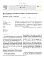
When the target reaches the thermal equilibrium status, the
atomic velocity distribution should follow the Maxwellian
distribution

Tk
mv
B
M
B
e
Tk
m
vP
2
2/3
2
2
2
4
−








=
π
π
(10)

where

M
P
is the probability for an atom moving with a velocity,
v
. The velocity distribution based on the simulation results as
well as the Maxwell's distribution, are shown in Fig. 1, which
indicates a good agreement between the two.

0 10
0
2 10
-3
4 10
-3
6 10
-3
8 10
-3
0 100 200 300 400 500
MD Simulation
Maxwell's Distribution
Probability
Velocity (m/s)

Figure 1. Comparison of the velocity distribution by the MD
simulation with the Maxwellian velocity distribution.

Figure 2 shows the lattice structure in the x-z plane when
the system is in thermal equilibrium. For the purpose of
illustration, only the atoms in the range of 120 << x nm and

6.120 << y
nm are plotted. It is seen that atoms are located
around their equilibrium positions, and the lattice structure is
preserved. It is also observed from Fig. 2 that at the top and the
5 Copyright © 2001 by ASME
bottom surfaces of the target, a few atoms have escaped due to
the free boundary conditions.

4
7
10
13
024681012
z (nm)
x (nm)

Figure 2. Structure of the target in the x-z plane within the range
of 120 << x nm and
6.120 << y
nm

III.2 Calculation of Thermophysical Properties
In order to check the validity of the simulation, thermal
physical properties including the specific heat at constant
pressure, the specific heat at constant volume, and the thermal
conductivity are calculated and compared with published data.
To calculate the specific heat at constant pressure, the
system is first equilibrated with periodical boundary conditions
in x and y directions, and free boundary conditions in the z
direction, which simulates a target in vacuum. A kinetic energy

of Tk
B
δ
⋅2/3 with 8=T
δ
is added to each atom and the
system is calculated for about 100 ps to reach a new thermal
equilibrium status with a final temperature increase of
T
∆
. The
specific heat is calculated as

)/(2/3 TmTkc
Bp
∆δ
⋅⋅= (11)

The specific heat at constant pressure (vacuum) is
calculated to be 787.8 J/kg·K at 51.476 K. This value is about
24% higher than the literature data, which is 637.5 J/kg·K [15].
This difference is mainly due to the free boundary conditions of
vacuum used in the MD simulation, while the experimental
results are for samples under atmospheric pressure. Under free
boundary conditions, atoms are easier to expand in space when
heated. Therefore, more heat is stored in the form of potential
energy and resulting in a larger specific heat.
The specific heat at constant volume is calculated in the
similar way as described above except that free boundary
conditions in the z direction are replaced with periodical

boundary conditions in order to keep the volume constant. The
specific heat at constant volume is calculated to be 576.0
J/kg·K, which is only 6% higher than the literature value of
543.5 J/kg·K [15]. This small difference might be due to the
potential function used in the calculation, which is more
suitable for argon in liquid state.
The thermal conductivity of argon is calculated as follows.
The target is first equilibrated with periodical boundary
conditions in x and y directions, and free boundary conditions
in the z direction. A constant heat flux q
′′
is applied to the
surface of the target by scaling velocities of atoms in cells on
the top surface, and the same amount of heat flux is dissipated
from the bottom of the target by scaling velocities of atoms in
cells at the bottom. The heat flux q
′′
is taken as
8
1083216.2 × W/m
2
, which induces a temperature difference of
about 5 K across the target. Figure 3 shows the temperature
distribution in the target when a heat flux is passing through. It
is seen that a linear temperature distribution is established in the
target due to the heat flux. The thermal conductivity k is
calculated as

x
T

q
k
∂∂
/
′′
−=
(12)

The thermal conductivity of the target is calculated to be
0.304 W/m·K, which is about 34% smaller than the
experimental value of 0.468 W/m·K. This large difference could
be due to the free boundary conditions used in the calculation
and possible errors in the potential function. Further work is
necessary to study the effects of boundary conditions and
different potential functions.

46
47
48
49
50
51
52
53
54
471013
Temperature (K)
z (nm)

Figure 3. Temperature distribution in the target subjected to a

constant heat flux

III.3 Laser Material Interaction
In laser material interaction, periodical boundary
conditions are assumed on surfaces in x and y directions, and
free boundary conditions on surfaces in the z direction. The
simulation corresponds to the problem of irradiating a block in
vacuum. The laser beam is uniform in space, and has a temporal
Gaussian distribution with a 5 ps FWHM centered at 10 ps. The
6 Copyright © 2001 by ASME
laser beam energy is absorbed exponentially in the target and
expressed as

τ
/)(zI
d
z
dI
−=
(13)

where I is the laser beam intensity, and
τ
is the characteristic
absorption depth, which is taken as 2.5 nm.

Laser Heating

The temperature distribution in the target illuminated with a
laser pulse of 0.03 J/m

2
is first calculated and compared with
finite difference results. With this laser fluence, only a
temperature increase is induced, and no phase change occurs.
Figure 4 shows the temperature distribution calculated using the
MD simulation and the finite difference method. In MD
simulations, temperature at different locations is calculated as
an ensemble average of a domain with thickness of 2.5
σ
in the z
direction. In the calculation using the finite difference method,
properties of the target obtained with the MD simulation are
used. It is observed from Fig. 4 that the results obtained from
the MD simulation show proper trends comparing with those by
the finite difference method. The difference between them is on
the same order of the statistic uncertainty of the MD simulation.
In other words, the continuum approach is still capable of
predicting the heating process induced by a picosecond laser
pulse.

Laser Induced Phase Change
In this section, various phenomena accompanying phase
change in an argon target illuminated with a laser pulse of 0.7
J/m
2
are investigated. The threshold fluence for ablation is also
studied.
For argon illuminated with a pulsed laser of 0.7 J/m
2
, a

series of snapshots of atomic positions at different times is
shown in Fig. 5. It is seen that until 10 ps, the lattice structure is
still preserved in the target. At about 10 ps, melting starts, and
the lattice structure is destroyed in the melted region and is
replaced by a random atomic distribution. After 20 ps, the solid
liquid interface stops moving into the target, and vaporized
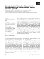
atoms are clearly seen. Figure 6 shows the distribution of
number density of atoms in space at different times, which
demonstrates the variation of solid structure during laser
heating. At the early stage of laser heating, the crystal structure
is preserved in the target, which is seen as the peak number
density of atoms on each lattice layer. Due to the increase of the
atomic kinetic energy in laser heating, atoms vibrate more in the
crystal region, causing a lower peak of the number density of
atoms and a wide distribution. As laser heating progresses, the
target is melted from its front surface, and the atomic
distribution becomes random. Therefore, the number density of
atoms becomes uniform over the melted region. However, no
clear interface is observed between the solid and the liquid.
Instead, the structure of solid and liquid co-exists within a
certain range between the solid and the liquid, which is shown
as the co-existence of the peak and the high base of the number
density of atoms. Evaporation happens at the surface of the
target, which reduces the number density of atoms significantly
at the location near the liquid surface.

48
50
52
54

56
MD simulation
Finite Difference
t=5 ps

50
52
54
56
MD simulation
Finite Difference
t=10 ps

50
52
54
56
MD simulation
Finite Difference
t=15 ps
Temperature (K)

50
52
54
56
MD simulation
Finite Difference
t=20 ps

50
52
54
56
MD simulation
Finite Difference
t=25 ps

50
52
54
56
MD simulation
Finite Difference
4 7 10 13
t=30 ps
z (nm)

Figure 4. Temperature distribution in the target illuminated with
a laser pulse of 0.03 J/m
2
.

In order to find out the rate of melting and evaporation,
criteria are needed to determine the solid-liquid and liquid-
vapor interfaces. For solid argon, the average number density of
atoms is
28
1052.2 × m
-3

with a distribution in space as shown in
Fig. 6. Owing to the lattice structure, the number density of
atoms is higher than the average value around the lattice layer
location. In this work, if the number density of atoms is higher
7 Copyright © 2001 by ASME
than
28
1052.2 × m
-3
, the material is treated as solid. At the front
of the melted region, it is seen from Fig. 6 that when the number
density of atoms is below
27
42.8 × m
-3
, a relatively sharp
decrease of the number density of atoms happens. Therefore,
when the number density of atoms is less than
27
1042.8 × m
-3
,
which is about one third of the number density in solid, the
material is assumed to be vapor. Although this criterion for
liquid-vapor interface is not quite rigorous due to the large
transition range from liquid to vapor, further study of the liquid-
vapor interface using radial distribution function shows that the
criterion used here gives a good approximation of the liquid-
vapor interface.

0
4
8
12
(t=5 ps)

0
4
8
12
(t=10 ps)

0
4
8
12
(t=15 ps)

0
4
8
12
(t=20 ps)

0
4
8
12
(t=25 ps)

0
4
8
12
357911131517
x (nm) (t=30 ps)
z (nm)

Figure 5. Snapshots of atomic positions in argon illuminated
with a laser pulse with a fluence of 0.7 J/m
2
.

Applying these criteria, transient locations of the solid-
liquid and liquid-vapor interfaces, as well as the velocity of
interfaces can be obtained and are shown in Fig. 7. It is
observed that melting and evaporation start at 10 ps, while laser
heating starts at around 5 ps. It is seen that the solid-liquid
interface moves into the solid owing to the melting of the solid,
and the liquid-vapor interface moves outward as the melted
region expands because liquid is less dense than solid. At about
20 ps, both solid-liquid and liquid-vapor interfaces stop
moving. The velocities of the interfaces are shown in Fig. 7b. It
is seen that the duration of the interface movement is about 10
ps, which is about the same as the laser pulse width. The highest
velocity of the liquid-vapor interface is about 200 m/s, close to
the equilibrium velocity (233.5 m/s) of the argon atom at the
boiling temperature. The highest velocity of the solid-liquid
interface is about 400 m/s, lower than the sound velocity (1501
m/s) in argon.

0.00
0.25
0.50
0.75
1.00
1.25
t=5 ps

0.00
0.25
0.50
0.75
1.00
1.25
t=10 ps
/m
3
)

0.00
0.25
0.50
0.75
1.00
1.25
t=15 ps
of Atoms (10
29

0.00
0.25
0.50
0.75
1.00
1.25
t=20 ps
Number Density

0.00
0.25
0.50
0.75
1.00
1.25
t=25 ps

0.00
0.25
0.50
0.75
1.00
1.25
3 5 7 9 11 13 15 17
t=30 ps
z (nm)

Figure 6. Distribution of number density of atoms at different
times in argon illuminated with a laser pulse of 0.7 J/m

2
.

The temperature distribution in argon at different times is
shown in Fig. 8. At 5 ps, laser heating just starts, and the target
has a spatially uniform temperature of about 50 K. Note that the
initial size of the target extends from 4.5 nm to 12.6 nm.
Melting starts at 10 ps as indicated in Fig. 7, and it is clear from
Fig. 8 that at this moment, the temperature is higher than the
melting and the boiling point in the heated region, and is even
close to the critical point. At 15 ps, a flat region in the
temperature distribution is observed around the location of 10
8 Copyright © 2001 by ASME
nm, which is the melting interface region. The temperature in
this flat region is around 90 K, which is higher than the melting
point, indicating superheating at the melting front.

9
10
11
12
13
14
15
16
0 5 10 15 20 25 30
Solid-liquid Interface
Liquid-vapor Interface
z (nm)
Time (ps)

(a)


-500
-250
0
250
500
0 5 10 15 20 25 30
Solid-liquid Interface
Liquid-vapor Interface
Velocity (m/s)
Time (ps)
(b)

Figure 7. (a) Positions (b) velocities of the solid-liquid interface
and the liquid-vapor interface in argon illuminated with a laser
pulse of 0.7 J/m
2
.

An interesting phenomenon is observed at 20 ps, shortly
after melting stops. At this moment, a minimum temperature is
observed at 9.5 nm. The reason for this temperature drop is not
known yet, and is still under investigation. This minimum
temperature disappears gradually due to heat transfer from the
surrounding higher temperature regions. It is worth noting that
results of superheating, as well as the lack of a sharp solid-
liquid interface as mentioned previously, could not be predicted
using the continuum approaches without assumptions.

40
60
80
100
120
140
3 5 7 9 11 13 15 17
t=5 ps
t=10 ps
t=15 ps
t=20 ps
t=25 ps
t=30 ps
Temperature (K)
z (nm)
T
m
T
b

Figure 8. Temperature distribution in argon illuminated with a
laser pulse of 0.7 J/m
2
.

The velocity distribution of vaporized atoms at different
times is shown in Fig. 9. At 10 ps, melting just starts, and the
average velocity of atoms is close to zero except those on the
surface, which have high kinetic energy due to the free

boundary condition. At 15 ps, a higher atomic velocity is
observed. At the vapor front, the velocity is close to 800 m/s,
while at locations near the surface, the vapor velocity is much
smaller. At 30 ps, non-zero velocities are only observed at
locations of 15 nm or further beyond the liquid-vapor interface
as indicated in Fig. 7. This shows evaporation from the liquid
surface is weak after laser heating stops.

-200
0
200
400
600
800
0 5 10 15 20
t=5 ps
t=10 ps
t=15 ps
t=20 ps
t=25 ps
t=30 ps
Average Velocity (m/s)
z (nm)

Figure 9. Spatial distribution of the average velocity in the z
direction in argon illuminated with a laser pulse of 0.7 J/m
2
.

9 Copyright © 2001 by ASME
0
1
2
3
0 5 10 15 20 25 30
Melting
Evaporation
Depth (nm)
Time (ps)
(a)

-100
0
100
200
300
400
0 5 10 15 20 25 30
Melting
Evaporation
Rate of Depth (m/s)
Time (ps)
(b)

Figure 10. (a) Depths of the solid melted and vaporized, and (b)
rate of melting and evaporation in argon illuminated with a laser
pulse of 0.7 J/m
2

.

0
1
2
3
0 0.2 0.4 0.6 0.8 1 1.2 1.4 1.6
Ablation Depth (nm)
Energy Fluence (J/m
2
)

Figure 11. The ablation depth induced by different laser
fluences in argon.


The depth of melting and vaporization, as well as the
melting and evaporation rates are shown in Fig. 10. It is seen
that the melting depth is much larger than the vaporization
depth. From Fig. 10b it is found that melting happens mostly
between 10 and 20 ps, while the evaporation process goes on
until 25 ps, then reduces to a lower level corresponding to
evaporation of liquid in vacuum. The depths of ablation induced
by different laser fluences are shown in Fig. 11.

IV. CONCLUSION
In this work, laser material interaction is studied using MD
simulations. Based on the results, the following conclusions are
obtained. First, during picosecond laser heating, the heat
transfer process predicted using the continuum approach agrees

with the result of the MD simulation. Second, when melting
happens, a transition region of about 1 nm, instead of a clear
interface is found between the solid and the liquid. During the
melting process, the solid-liquid interface moves at almost a
constant velocity much lower than the local sound velocity,
while the liquid-vapor interface moves with a velocity close to
the local equilibrium atomic velocity. At the solid-liquid
interface, superheating is observed. Finally, the laser ablated
material is found to move out of the target with a velocity of
about a thousand meters per second.

ACKNOWLEDGMENTS
Support to this work by the National Science Foundation
(CTS-9624890) is gratefully acknowledged.

REFERENCES
1. Shibahara, M., and Kotake, S., 1997, "Quantum
Molecular Dynamics Study on Light-to-heat Absorption
Mechanism: Two Metallic Atom System," International Journal
of Heat and Mass Transfer, 40, pp. 3209-3222.
2. Shibahara, M., and Kotake, S., 1998, "Quantum
Molecular Dynamics Study of Light-to-heat Absorption
Mechanism in atomic Systems," International Journal of Heat
and Mass Transfer, 41, pp. 839-849.
3. Häkkinen, H., and Landman, U., 1993, "Superheating,
Melting, and Annealing of Copper Surfaces," Physical Review
Letters, 71, pp. 1023-1026.
4. Anisimov, S. I., Kapeliovich, B. L., Perel'man, T. L.,
1974, "Electron Emission from Metal Surfaces Exposed to
Ultra-short Laser Pulses," Soviet Physics, JETP, 39, pp. 375-

377.
5. Kotake, S., and Kuroki, M., 1993, "Molecular Dynamics
Study of Solid Melting and Vaporization by Laser Irradiation,"
International Journal of Heat and Mass Transfer, 36, pp. 2061-
2067.
6. Herrmann, R. F. W., and Campbell, E. E. B., 1998,
"Ultrashort Pulse Laser Ablation of Silicon: an MD Simulation
Study," Applied Physics A, 66, pp. 35-42.
10 Copyright © 2001 by ASME
7. Zhigilei, L. V., Kodali, P. B. S., and Garrison, J., 1997,
"Molecular Dynamics Model for Laser Ablation and Desorption
of Organic Solids," Journal of Physical Chemistry B, 101, pp.
2028-2037.
8. Zhigilei, L. V., Kodali, P. B. S., and Garrison, J., 1998,
"A Microscopic View of Laser Ablation," Journal of Physical
Chemistry B, 102, pp. 2845-2853.
9. Ohmura, E., Fukumoto, I., and Miyamoto, I., 1999,
"Modified Molecular Dynamics Simulation on Ultrafast Laser
Ablation of Metal," the International Congress on Applications
of Lasers and Electro-Optics, 1999, pp. 219-228.
10. Girifalco, L. A., and Weizer, V. G., 1959, "Application
of the Morse Potential Function to Cubic Metals," Physical
Review, 114, pp. 687-690.
11. Etcheverry, J. I., and Mesaros, M., 1999, "Molecular
Dynamics Simulation of the Production of Acoustic Waves by
Pulsed Laser Irradiation," Physical Review B, 60, pp. 9430-
9434.
12. Allen, M. P. and Tildesley, D. J., 1987, Computer
Simulation of Liquids, Clarendon Press, Oxford.
13. Broughton, J. Q. and Gilmer, G. H., 1983, "Molecular

Dynamics Investigation of the Crystal-fluid Interface. I. Bulk
Properties," Journal of Chemical Physics, 79, pp. 5095-5104.
14. Berendsen, H. J. C, Postma, J. P. M, van Gunsteren, W.
F., DiNola, A., and Haak, J. R., 1984, "Molecular Dynamics
with Coupling to an External Bath," Journal of Chemical
Physics, 81, pp. 3684-90.
15. Peterson, O. G., Batchelder, D. N., and Simmons, R. O.,
1966, "Measurements of X-Ray Lattice Constant, Thermal
Expansivity, and Isothermal Compressibility of Argon Crystals,"
Physical Review, 150, pp. 703-711