Wavelets
Bạn đang xem bản rút gọn của tài liệu. Xem và tải ngay bản đầy đủ của tài liệu tại đây (1.54 MB, 109 trang )
Wavelets (Chapter 7)
CS474/674 – Prof. Bebis
STFT (revisited)
•
Time/Frequency localization depends on window size.
•
Once you choose a particular window size, it will be the same for all frequencies.
•
Many signals require a more flexible approach - vary the window size to determine more
accurately either time or frequency.
The Wavelet Transform
•
Overcomes the preset resolution problem of the STFT by using a variable length window:
–
Use narrower windows at high frequencies for better time
resolution.
–
Use wider windows at low frequencies for better frequency
resolution.
The Wavelet Transform (cont’d)
Wide windows do not provide good localization
at high frequencies.
The Wavelet Transform (cont’d)
Use narrower windows at high frequencies.
The Wavelet Transform (cont’d)
Narrow windows do not provide good localization
at low frequencies.
The Wavelet Transform (cont’d)
Use wider windows at low frequencies.
What are Wavelets?
•
Wavelets are functions that “wave” above and below the x-axis, have (1) varying
frequency, (2) limited duration, and (3) an average value of zero.
•
This is in contrast to sinusoids, used by FT, which have infinite energy.
Sinusoid Wavelet
What are Wavelets? (cont’d)
•
Like sines and cosines in FT, wavelets are used as basis functions ψk(t) in representing
other functions f(t):
•
Span of ψk(t): vector space S containing all functions f(t) that can be represented by ψk(t).
( ) ( )
k k
k
f t a t
ψ
=
∑
What are Wavelets? (cont’d)
•
There are many different wavelets:
Morlet
Haar
Daubechies
(dyadic/octave grid)
What are Wavelets? (cont’d)
( )
jk
t
ψ
=
What are Wavelets? (cont’d)
time localization
scale/frequency
localization
( )
/2
( ) 2 2
j j
jk
t t k
ψ ψ
= −
j
Continuous Wavelet Transform (CWT)
( )
1
( , )
t
t
C s f t dt
s
s
τ
τ ψ
∗
−
=
÷
∫
Continuous Wavelet Transform
of signal f(t)
translation parameter,
measure of time
scale parameter
(measure of frequency)
Mother wavelet
(window)
normalization
constant
Forward
CWT:
Scale = 1/j = 1/Frequency
CWT: Main Steps
1. Take a wavelet and compare it to a section at the start
of the original signal.
2. Calculate a number, C, that represents how closely
correlated the wavelet is with this section of the
signal. The higher C is, the more the similarity.
CWT: Main Steps (cont’d)
3. Shift the wavelet to the right and repeat steps 1 and 2 until you've covered the whole
signal.
CWT: Main Steps (cont’d)
4. Scale the wavelet and repeat steps 1 through 3.
5. Repeat steps 1 through 4 for all scales.
Coefficients of CTW Transform
( )
1
( , )
t
t
C s f t dt
s
s
τ
τ ψ
∗
−
=
÷
∫
•
Wavelet analysis produces a time-scale view of the input
signal or image.
Continuous Wavelet Transform (cont’d)
•
Inverse CWT:
1
( ) ( , ) ( )
s
t
f t C s d ds
s
s
τ
τ
τ ψ τ
−
=
∫∫
double integral!
FT vs WT
weighted by F(u)
weighted by C(τ,s)
Properties of Wavelets
•
Simultaneous localization in time and scale
- The location of the wavelet allows to explicitly represent
the location of events in time.
- The shape of the wavelet allows to represent different
detail or resolution.
Properties of Wavelets (cont’d)
•
Sparsity: for functions typically found in practice, many of the coefficients in a
wavelet representation are either zero or very small.
•
Linear-time complexity: many wavelet transformations can be accomplished in O(N)
time.
1
( ) ( , ) ( )
s
t
f t C s d ds
s
s
τ
τ
τ ψ τ
−
=
∫∫
Properties of Wavelets (cont’d)
•
Adaptability: wavelets can be adapted to represent a wide variety of functions (e.g.,
functions with discontinuities, functions defined on bounded domains etc.).
–
Well suited to problems involving images, open or
closed curves, and surfaces of just about any variety.
–
Can represent functions with discontinuities or corners
more efficiently (i.e., some have sharp corners
themselves).
Discrete Wavelet Transform (DWT)
( ) ( )
jk jk
k j
f t a t
ψ
=
∑∑
( )
/2
( ) 2 2
j j
jk
t t k
ψ ψ
= −
(inverse DWT)
(forward DWT)
where
*
( ) ( )
jk
jk
t
a f t t
ψ
=
∑
DFT vs DWT
•
FT expansion:
•
WT expansion
or
one parameter basis
( ) ( )
l l
l
f t a t
ψ
=
∑
( ) ( )
jk jk
k j
f t a t
ψ
=
∑∑
two parameter basis
Multiresolution Representation using
( ) ( )
jk jk
k j
f t a t
ψ
=
∑ ∑
( )f t
( )
jk
t
ψ
j
fine
details
coarse
details
wider, large translations