Astm e 1636 10
Bạn đang xem bản rút gọn của tài liệu. Xem và tải ngay bản đầy đủ của tài liệu tại đây (240.32 KB, 8 trang )
Designation: E1636 − 10
Standard Practice for
Analytically Describing Depth-Profile and Linescan-Profile
Data by an Extended Logistic Function1
This standard is issued under the fixed designation E1636; the number immediately following the designation indicates the year of
original adoption or, in the case of revision, the year of last revision. A number in parentheses indicates the year of last reapproval. A
superscript epsilon (´) indicates an editorial change since the last revision or reapproval.
priate safety and health practices and determine the applicability of regulatory limitations prior to use.
1. Scope
1.1 This practice describes a systematic method for analyzing depth-profile and linescan data and for accurately characterizing the shape of an interface region or topographic feature.
The profile data are described with an appropriate analytic
function, and the parameters of this function define the
position, width, and any asymmetry of the interface or feature.
The use of this practice is recommended in order that the
shapes of composition profiles of interfaces or of linescans of
topographic features acquired with different instruments or
techniques can be unambiguously compared and interpreted.
2. Referenced Documents
2.1 ASTM Standards:2
E673 Terminology Relating to Surface Analysis (Withdrawn
2012)3
E1127 Guide for Depth Profiling in Auger Electron Spectroscopy
E1162 Practice for Reporting Sputter Depth Profile Data in
Secondary Ion Mass Spectrometry (SIMS)
E1438 Guide for Measuring Widths of Interfaces in Sputter
Depth Profiling Using SIMS
1.2 This practice is intended to be used for two purposes.
First, it can be used to describe the shape of depth-profiles
obtained at an interface between two dissimilar materials that
might be measured by common surface-analysis techniques
such as Auger electron spectroscopy, secondary-ion mass
spectrometry, and X-ray photoelectron spectroscopy. Second, it
can be used to describe the shape of linescans across a
detectable topographic feature such as a step or a feature on a
surface that might be measured by a surface-analysis
technique, scanning electron microscopy, or scanning probe
microscopy. The practice is particularly valuable for determining the position and width of an interface in a depth profile or
of a feature on a surface and in assessments of the width as an
indication of the sharpness of the interface or feature (a
characteristic of the material system being measured) or of the
achieved depth resolution of the profile or the lateral resolution
of the linescan (a characteristic of the particular analytical
technique and instrumentation).
2.2 ISO Standards:4
ISO 18115 Surface Chemical Snalysis – Vocabulary, 2001;
Amd. 1:2006, Amd. 2:2007
ISO 18516 Surface Chemical Analysis – Auger Electron
Spectroscopy and X-Ray Photoelectron Spectroscopy –
Determination of Lateral Resolution, 2006
3. Terminology
3.1 Definitions—For definitions of terms used in this
practice, see Terminology E673 and ISO 18115.
3.2 Definitions of Terms Specific to This Standard:
3.2.1 Throughout this practice, three regions of a sigmoidal
profile will be referred to as the pre-interface, interface, and
post-interface regions. These terms are not dependent on
whether a particular interface or feature profile is a growth or
a decay curve. The terms pre- and post- are taken in the sense
of increasing values of the independent variable X, the depth
(for a depth profile) or the lateral position on the surface (for a
linescan).
1.3 The values stated in SI units are to be regarded as
standard. No other units of measurement are included in this
standard.
1.4 This standard does not purport to address all of the
safety concerns, if any, associated with its use. It is the
responsibility of the user of this standard to establish appro-
2
For referenced ASTM standards, visit the ASTM website, www.astm.org, or
contact ASTM Customer Service at For Annual Book of ASTM
Standards volume information, refer to the standard’s Document Summary page on
the ASTM website.
3
The last approved version of this historical standard is referenced on
www.astm.org.
4
Available from International Organization for Standardization (ISO), 1, ch. de
la Voie-Creuse, Case postale 56, CH-1211, Geneva 20, Switzerland, http://
www.iso.ch.
1
This practice is under the jurisdiction of ASTM Committee E42 on Surface
Analysis and is the direct responsibility of Subcommittee E42.08 on Ion Beam
Sputtering.
Current edition approved Jan. 1, 2010. Published March 2010. Originally
approved in 1999. Last previous version approved in 2004 as E1636 – 04. DOI:
10.1520/E1636-10.
Copyright © ASTM International, 100 Barr Harbor Drive, PO Box C700, West Conshohocken, PA 19428-2959. United States
1
E1636 − 10
5.5 Many attempts have been made to characterize interface
profiles with general functions (such as polynomials or error
functions) but these have suffered from instabilities and an
inability to handle poorly structured data. Choice of the logistic
function along with a specifically written least-squares procedure (described in Appendix X1) can provide statistically
evaluated parameters that describe the width, asymmetry, and
depth of interface profiles or linescans in a reproducible and
unambiguous way.
4. Summary of Practice
4.1 Depth-profile data for an interface (that is, signal intensity or composition versus depth) or linescan data (that is,
signal intensity or composition versus position on a surface)
are fitted to an analytic function, an extended form of the
logistic function, in order to describe the shape of such
profiles.5,6 Least-squares fitting techniques are employed to
determine the values of the parameters of this extended logistic
function that characterize the shape of the interface. The
interface width, depth or position, and asymmetry are determined from these parameters.
6. Description of the Analysis
6.1 Logistic Function Data Analysis—The logistic function
was first named and applied to population growth in the 20th
century by Verhulst.7 In its simplest form, this function may be
written as:
5. Significance and Use
5.1 Information on interface composition is frequently obtained by measuring surface composition while the specimen
material is gradually removed by ion bombardment (see Guide
E1127 and Practice E1162). In this way, interfaces are revealed
and characterized by the measurement of composition versus
depth to obtain a sputter-depth profile. The shape of such
interface profiles contains information about the physical and
chemical properties of the interface region. In order to accurately and unambiguously describe this interface region and to
determine its width (see Guide E1438), it is helpful to define
the shape of the entire interface profile with a single analytic
function.
Y5
1
11e 2x
(1)
in which Y progresses from 0 to 1 as X varies from −∞ to +∞.
The differential equation generating this function is:
dY/dX 5 Y ~ 1 2 Y !
(2)
and in this form describes a situation where a measurable
quantity Y grows in proportion to Y and in proportion to finite
resources required by Y. Appropriate to an interface, the
propensity for change in the fractional composition of a species
at a particular boundary is proportional to the concentration of
that species at the boundary and the concentration of the other
species at the adjacent boundary. The logistic function as a
distribution function and growth curve has been extensively
reviewed by Johnson and Kotz.8 Interface or linescan profile
data are usefully fitted to an extended form of the logistic
function:
5.2 Interfaces in depth profiles from one semi-infinite medium to another generally have a sigmoidal shape characteristic
of the cumulative logistic distribution. Use of such a logistic
function is physically appropriate and is superior to other
functions (for example, polynomials) that have heretofore been
used for interface-profile analysis in that it contains the
minimum number of parameters for describing interface
shapes.
Y 5 @ A1A s ~ X 2 X 0 ! # / ~ 11e z !
5.3 Measurements of variations in signal intensity or surface
composition as a function of position on a surface give
information on the shape of a step or topographic feature on a
surface or on the sharpness of an interface at a phase boundary.
The shapes of steps or other features on a surface can give
information on the lateral resolution of a surface-analysis
technique if the sample being measured has sufficiently sharp
edges (see ISO 18516). Similarly, the shapes of compositional
variations across a surface can give information on the physical
and chemical properties of the interface region (for example,
the extent of mixing or diffusion across the interface). It is
convenient in these applications to describe the measured
linescan profile with an appropriate analytic function.
(3)
1 @ B1B s ~ X 2 X 0 ! # / ~ 11e 2z !
where:
z 5 ~ X 2 X 0 ! /D
(4)
D 5 2D 0 / @ 11e Q ~ X2X 0 ! #
(5)
and:
6.1.1 Y is a measured signal (for example, from a surfaceanalysis instrument, a scanning electron microscope, or a
scanning probe microscope) or a measure of the elemental
surface concentration of one of the components and X, the
independent variable, is a measure of the sputtered depth,
usually expressed as a sputtering time, or lateral position on the
surface. Pre-interface and post-interface signals or surface
concentrations are described by the parameters A and B,
respectively, and the parameters As and Bs are introduced to
account for any time-dependent instrumental effects or otherwise to better describe the shape of the measured profile. X0 is
the midpoint of the interface region (depth or time for a profile
or of position for a linescan). The scaling factor D0 is a
5.4 Although the logistic distribution is not the only function that could be used to describe measured linescans, it is
physically plausible and it has the minimum number of
parameters for describing such linescans.
5
Kirchhoff, W. H., Chambers, G. P., and Fine, J., “An Analytical Expression for
Describing Auger Sputter Depth Profile Shapes of Interfaces,” Journal of Vacuum
Science and Technology A, Vol 4, 1986, p. 1666.
6
Wight, S. A. and Powell, C. J., “Evaluation of the Shapes of Auger- and
Secondary-Electron Line Scans across Interfaces with the Logistic Function,”
Journal of Vacuum Science and Technology A, Vol 24, 2006, p. 1024.
7
Verhulst, P. F., Acad. Brux, Vol 18 , 1845, p. 1.
Johnson, N. L., and Kotz, S., Distributions in Statistics: Continuous Univariate
Distributions, Chapter 22, Houghton Mifflin Co., Boston, 1970.
8
2
E1636 − 10
6.3.1 The fitting can also be done in Excel, using the solver
option to determine the variables A, B, As, Bs, X0, D0, and Q.
Write the definition of the logistic function (Eq 3-5) in Excel
and calculate its values as a function of X. If the exponential
function ez produces overflow when z > 709, this problem can
easily be circumvented by writing EXP (min (z, 709)) instead
of EXP(z).
6.3.2 The fitting can also be done with any suitable nonlinear least-squares software that is available.
characteristic depth for sputtering through the interface region
of a depth profile or a characteristic width for a linescan; Q, an
asymmetry parameter, is a measure of the difference in
curvature in the pre- and post-interface ends of the interface
region. Conventional measures of the interface width can be
determined from D0 and Q. Fig. 1 shows examples of profile
shapes from Eq 3-5 for illustrative values of D0 and Q.5
6.2 Fitting of interface-profile data to the above function, Eq
3, can be accomplished by using least-squares techniques.
Because these equations are non-linear functions of the three
transition-region parameters, X 0, D0, and Q, the least-squares
fit requires an iterative solution. Consequently, Y, as expressed
by Eq 3, can be expanded in a Taylor series about the current
values of the parameters and the Taylor series terminated after
the first (that is, linear) term for each parameter.
Y(obs) − Y(calc) is fitted to this linear expression and the
least-squares routine returns the corrections to the parameters.
The parameters are updated and the procedure is repeated until
the corrections to the parameters are deemed to be insignificant
compared to their standard deviations. Values for interface
width, depth, and asymmetry can be calculated from the
parameters of the fitted logistic function. The iterative solution
also requires a robust means for making initial estimates of the
parameter values.
7. Interpretation of Results
7.1 The seven parameters necessary to characterize the
interface-profile shape are determined by a least-squares fit of
the interface data to the extended logistic function. These
parameters are related to the three distinct regions of the
interface profile. Two parameters, an intercept A and a slope As
are necessary to define the pre-interface asymptote while two
more, B and Bs, define the post-interface asymptote. For the
analysis of many interface profiles, it may be satisfactory to
assume that both of the slope parameters, As and Bs, are zero.
Two more parameters, D0 and X0, define the slope and position
of the transition region. In addition, an asymmetry parameter Q
that causes the width parameter to vary logistically from 0 to
2D0, is introduced as a measure of the difference in curvature
in the pre- and post-transition ends of the transition region. If
Q < 0, the pre-transition region has the greatest (sharpest)
curvature. If Q > 0, the post-transition region has the greatest
curvature. If Q = 0, D = D0 and the transition profile is
symmetric. The parameter Q has the dimensions of 1⁄ X whereas
6.3 Implementation of this procedure can be readily accomplished by making use of a specialized computer algorithm and
supporting software (logistic function profile fit (LFPF)) developed specifically for this application and described in
Appendix X1.
FIG. 1 Plot of Eq 3-5 Showing Relative Intensity as a Function of Relative Position X with A = As = Bs = X0 = 0, B = 100, D0 = 10 nm, and
the Indicated Values of Q (from the paper referenced in Footnote 5)
3
E1636 − 10
NOTE 1—The solid lines are the profiles calculated from the least-squares parameters shown in Table 2.
FIG. 2 Results of the Least-Squares Fit of the Simulated Cr and Ni Auger Intensities (Symbols) in Table 1 to the Extended Logistic
Function of Eq 3
D0 has the dimensions of X. The product QD0 is dimensionless
and is a measure of the asymmetry of the profile independent
of its width. If the absolute magnitude of QD0 is less than 0.1,
the asymmetry in the transition profile should be barely
discernible. Fig. 1 shows illustrative plots of the logistic
function (Eq 3-5) for values of QD0 0, 0.05, 0.1, 0.2, and 0.5.
84 % points of the interface more complicated. In particular,
for fractions f and (1 − f) of completion of the interface
transition:
X f 5 X 0 12 D 0 1n @ f/ ~ 1 2 f ! # / @ 11e Q ~ X f 2X 0 ! #
(7)
7.2 The final results should include the calculated values of
Y and associated statistics, the values of the determined
parameters and their uncertainties, and statistics related to the
overall quality of the least-squares fit.
X ~ 12f ! 5 X 0 12 D 0 1n @ ~ 1 2 f ! /f # / @ 11e Q ~ X 12f 2X 0 ! #
(8)
and:
Xf and X(1−f) (which appear on both sides of Eq 7 and Eq 8)
can be evaluated most readily by Newton’s method of successive approximations.
7.3 The width of the interface region, If, is the depth (time)
or distance required for the decay or growth curve to progress
from a fraction f of completion to (1 − f) of completion. For the
case where Q = 0, If is proportional to D0 and is given by the
simple formula:
I f 5 2D 0 1n @ ~ 1 2 f ! /f #
8. Reporting of Results
8.1 Interface profile shapes can be accurately characterized
by the extended logistic function and its parameters. Results of
such interface analysis should report these parameters (X0, D0,
and Q) together with their uncertainties, the standard deviation
of the fit, and an interface width obtained from D0 and Q that
is based on an accepted definition (for example, 16 % to 84 %
signal or concentration change; see also ISO 18516).
(6)
so that, for example, the traditional 16 % to 84 % interface
width is 3.32 D0. Similarly, the interface widths determined
from the 10 % to 90 %, 12 % to 88 %, 20 % to 80 %, and 25 %
to 75 % intensity changes are 4.39D0, 3.99D0, 2.77D0, and
2.20D0, respectively.
8.2 The sputtered depth, X, is often difficult to determine
experimentally so that depth profile data are normally acquired
with time as the independent variable. This sputtered time can
be referenced with respect to a removal time obtained with a
7.4 Introduction of the asymmetry parameter Q into the
extended logistic function makes the calculation of the 16 % to
4
E1636 − 10
TABLE 1 Simulated Auger Intensities for a Cr/Ni Interface to be
Used for Comparison of Computational Approaches
calibrated sputtering standard under the same sputtering conditions of ion energy, beam angle, current density, etc., as the
interface measurement itself. In this way, time can be transformed into an equivalent depth derived from a standard
material and this equivalent depth should be used in reporting
the interface parameters and analysis results. Sputtering standards are available from the National Institute of Standards and
Technology9 (SRM 2135c), from the European Institute for
Reference Materials and Measurements10 (BCR 261), and from
the Surface Analysis Society of Japan11 (a multilayer GaAs/
AlAs superlattice material).
NOTE 1—The Cr and Ni intensities have been normalized to range
between 0 and 1.
Time (min)
Cr Intensity
Ni Intensity
77.5
80.0
82.5
85.0
57.5
90.0
92.5
95.0
97.5
100.0
102.5
105.0
107.5
110.0
112.5
115.0
117.5
120.0
122.5
125.0
127.5
130.0
132.5
135.0
137.5
140.0
142.5
145.0
147.5
150.0
0.9932
0.9796
0.9933
0.9923
0.9849
0.9957
0.9963
1.0000
0.9930
0.9674
0.9026
0.7721
0.5618
0.3605
0.1991
0.1199
0.0596
0.0436
0.0230
0.0209
0.0148
0.0082
0.0157
0.0113
0.0065
0.0080
0.0118
0.0221
0.0000
0.0048
0.0155
0.0158
0.0000
0.0113
0.0159
0.0121
0.0009
0.0077
0.0313
0.0578
0.1352
0.3302
0.5464
0.7146
0.8437
0.9189
0.9367
0.9628
0.9825
0.9839
0.9964
0.9764
0.9793
0.9798
0.9926
0.9871
0.9809
1.0000
0.9862
0.9979
9. Example of Interface Profile Data Analysis Using the
Method Suggested
9.1 Depth-profile data obtained at an interface between
chromium (Cr) and nickel (Ni) have been analyzed by fitting
the extended logistic function to these data using least-squares
techniques.5 An analysis is reported in this standard of simulated data, based on the parameter values obtained from
measurements of the Cr/Ni SRM available from NIST.9 The
simulated data consist of normalized Auger spectral intensities
and include random, normal errors of magnitude comparable to
those obtained from the actual Cr/Ni measurements. The
simulated data are given in Table 1 and the results of the
analyses of the Cr and Ni simulated Auger intensities are given
in Table 2 and Fig. 2. The data in Table 1 can and should be
used as a basis for comparison of different algorithms. The
uncertainties presented for the parameters in Table 2 represent
95 % confidence limits assuming a normal distribution of
errors.
TABLE 2 Parameter Values From the Least-Squares Fit of the
Data in Table 1 to the Extended Logistic Function of Eq 3
10. Keywords
NOTE 1—Uncertainties represent 95 % confidence levels.
Parameter
A
As
B
Bs
X0 (min)
D0 (min)
Q (min-1)
Residual Standard
Deviation, σ
Confidence Limits
for σ
Cr
(Disappearance)
Ni
(Appearance)
1.009 ± 0.0154
0.000756 ± 0.000688
0.0103 ± 0.0168
-0.000049 ± 0.000519
108.132 ± 0.153
2.846 ± 0.108
-0.0341 ± 0.0175
0.0046 ± 0.0231
-0.00028 ± 0.00107
0.9888 ± 0.0258
0.00004 ± 0.00077
106.985 ± 0.231
2.801 ± 0.167
-0.0445 ± 0.0276
0.005567
0.008481
0.004502 < σ < 0.007379
0.006858 < σ < 0.01124
10.1 depth-profile interface data; linescan interface data;
logistic function
9
Information on standard reference materials from the National Institute of
Standards and Technology (NIST) is available from 100 Bureau Dr., Stop 1070,
Gaithersburg, MD 20899-1070, />referencematerials/index.cfm.
10
Information on certified reference materials from the European Institute for
Reference Materials and Measurements is available from European Commission,
Joint Research Centre, Institute for Reference Materials and Measurements,
Retieseweg 111, B-2440 Geel, Belgium, .
11
Information on the GaAs/AlAs certified reference material can be obtained
from the Surface Analysis Society of Japan at />
5
E1636 − 10
APPENDIX
(Nonmandatory Information)
X1. FITTING OF DEPTH PROFILE AND LINESCAN DATA TO THE LOGISTIC FUNCTION BY MEANS OF A
SPECIALIZED COMPUTER ALGORITHM, LOGISTIC FUNCTION PROFILE FIT (LFPF)
data consist of more than three values in each of the asymptotic
regions and five values in the interface region.
X1.3.4 LFPF provides statistical uncertainties on the parameters of the logistic function allowing assessment and comparison of data quality from different laboratories.
X1.1 Scope
X1.1.1 Appendix X1 describes a specialized computer algorithm and supporting software (LFPF) developed for the
fitting of depth profile and linescan interface data to the
extended logistic function in order to determine the parameters
of this fitted function. These parameters characterize the shape
of the interface region and so define the interface width, its
asymmetry, and its depth from the original surface or its width
along a scanned line.
X1.4 Description of the Fitting Procedure Used in LFPF
X1.4.1 Data in the form of X, Y pairs are fit by the method
of least-squares to the extended logistic function:
Y 5 @ A1A s ~ X 2 X 0 ! # / ~ 11e z !
X1.2 Significance and Use
(X1.1)
1 @ B1B s ~ X 2 X 0 ! # / ~ 11e 2z !
X1.2.1 LFPF has been developed to fit interface profile data
to the extended logistic function. The specifically written
least-squares procedure used in LFPF results in a rapid and
reliable analysis. An important feature of LFPF is that it does
not require initial estimates to be made of the parameters; it is,
therefore, simple and easy to use and can run without operator
intervention. LFPF is robust in handling a wide variety of data
of sigmoidal character and can deal effectively with extremely
sharp profiles, noisy data, and incomplete profiles. It can also
identify pronounced outliers.
where:
z 5 ~ X 2 X 0 ! /D, and D 5 2D 0 / @ 1 1 e Q ~ X 2 X 0 ! #
(X1.2)
X1.4.1.1 Because these equations are non-linear functions
of the three interface region parameters, X0, D0, and Q, the
least-squares fit requires an iterative solution. Consequently, Y,
as expressed above is expanded in a Taylor series about the
current values of the parameters and the Taylor series is
terminated after the first (that is, linear) term for each parameter. Yobs − Ycalc is fit to this linear expression and the
least-squares routine returns the corrections to the parameters.
The parameters are updated and the procedure is repeated until
the corrections to the parameters are deemed to be insignificant
compared to their standard deviations.
X1.4.2 Initial estimates of the values of the parameters are
calculated in LFPF automatically by one of three methods,
selected because they were found to be least prone to false
starts in situations of poorly structured data. The user has some
control over the calculation of initial estimates in cases of
poorly structured data.
X1.4.3 The Least-Square Analysis—A cycle of up to p
iterations is executed in which, at the end of each iteration, the
parameters are updated before the next iteration is performed.
The number of iterations p is chosen on the basis of experience
with particular classes of data. If p is selected to be a prime
number, oscillations between two or three local minima can be
identified by performing repeated multiples of p iterations.
Generally, if convergence takes longer than eleven iterations,
the solution is unstable in the sense that all of the parameters
cannot be determined from the data. In most cases, instability
of the fit can be interpreted by the program and the source of
the instability removed by varying one fewer parameter in the
least-squares fit. Messages keep the user informed of these
situations. The confidence limits for the logistic curve calculated from the parameters of the least-squares fit are directly
determined in LFPF.
X1.4.4 Situations with few data in the transition region can
be accommodated by LFPF but with some loss of statistical
significance.
X1.2.2 LFPF has been extensively tested on a variety of
interface profile data; it has been found able to fit such data to
the extended logistic function to within the measurement
uncertainty.
X1.2.3 LFPF is a suitable implementation procedure for use
with this practice.
X1.3 Description of the Procedure, LFPF
X1.3.1 LFPF has been written in Microsoft Visual Basic.Net, an object oriented programming language that makes full
use of the Microsoft Windows graphical user interface. It has
been tested and found to run satisfactorily on computers using
Microsoft Windows XP and Vista operating systems.
X1.3.2 LFPF is available for download together with accompanying documentation and instructions for use from
NIST.12
X1.3.3 LFPF operates on ASCII text files created by the
user or data entered directly into the program from the
keyboard by the user. The data is in the form of tables whose
rows consist of an independent variable, X, and up to 4
corresponding values of a dependent variable, Y, or a weighting
factor to be used in the least squares fit, or a combination
thereof. While the program can analyze poorly structured data,
the statistics provided by the program are most reliable if the
12
The LFPF software and its documentation can be downloaded from the web
site of the Surface and Microanalysis Science Division of NIST at http://
www.nist.gov/cstl/surface/lfpf.cfm.
6
E1636 − 10
functionality, program outputs, and the full mathematical
description of the analysis suitable for designing a similar
program.
X1.4.5 Post-Fitting Tests—Following the cycle of p
iterations, several tests are performed to judge the quality of
the fit, to test the assumption of the determinability of X0, D0,
and Q, and the determinability of the asymptotic parameters A
s, Bs. If a test is failed, the analysis is repeated holding certain
parameters constant. Analysis notes provided by the program
describe actions taken by the program.
X1.4.5.1 The philosophy underlying the performance of the
post-fitting tests is that the parameters As, Bs, and Q are of less
interest in the analysis of the logistic profile than the parameters D0 and X0. In general (but not always), the former are of
a heuristic nature and have little basis in the choice of the
logistic function as a descriptor of an interface profile.
X1.5.3 Sample data files of test data, including the data file
described above in this practice, accompany the program and
may be used to evaluate program performance as well as for
familiarization in the use of LFPF.
X1.6 Results of the Analysis
X1.6.1 The final results of an analysis of a depth profile or
a linescan obtained with LFPF include the original data, the
calculated values of Y and associated statistics, the values of
the determined parameters and their uncertainties, and statistics
related to the overall quality of the least-squares fit.
X1.4.6 Outlier Identification and Rejection—If directed to
do so, LFPF will, following completion of analysis, identify
outliers based on the assumption of a normal distribution of
errors in the data and the confidence level specified by the user
(the default being 95%.) The standardized residuals are used
for the identification of the outliers. A standardized residual is
the number of standard deviations by which Yobs − Ycalc differs
from its expected value of zero, that is, the value of Yobs − Ycalc
divided by the standard deviation of Yobs − Ycalc.
X1.6.2 Use of these parameters to characterize the interface
profile has been described in Section 7 of this practice.
X1.7 Summary Demonstration of LFPF
X1.7.1 On initiating the program, the user is presented with
instructions for entering profile data to be analyzed.
X1.7.2 After data entry and, if necessary, editing, a graph of
the data is displayed along with “buttons” for initiating the
analysis, text boxes for setting program operation parameters,
a list of the original data, and a table of parameters to be varied.
Following the least squares fit, the profile calculated from the
least squares fit parameters is drawn through the data, the
values of the parameters along with their uncertainties are
displayed along with the overall statistics of the least squares fit
and additional information about the analysis is printed in a
text box labeled “Analysis Notes” as in Fig. X1.1:
X1.4.7 Confidence Limits and Error Bars—If directed to do
so, LFPF will, following completion of analysis, display error
bars equal to the confidence limits for each of the data or draw
confidence intervals for the least squares profile, or both.
X1.5 Analysis Procedure Using LFPF
X1.5.1 LFPF is used in an interactive configuration for the
analysis of interface data. With the graphical user interface, the
user can select the following:
X1.5.1.1 Which data files are to be analyzed,
X1.5.1.2 Which parameters are to be varied,
X1.5.1.3 Which data are to be included in the analysis, and
X1.5.1.4 The results of a least-squares fit (the graphical
display or the parameter table, or both) can be saved to the
Windows clipboard for subsequent pasting into word processors.
X1.7.3 The analysis displayed in Fig. X1.1 also included a
request to identify outliers, that is, data lying outside the 95 %
(default value) confidence limits. This analysis also includes
the statistics that would result if the outlier were excluded from
the analysis.
X1.7.4 Many optional features including copying results,
displaying additional statistics, remembering and displaying a
previous analysis are available on the drop down menus.
X1.5.2 A user manual is included with the downloaded
program and contains detailed descriptions of the program
7
E1636 − 10
NOTE 1—The X-axis is sputtering time and the Y-axis is the normalized Cr Auger signal.
FIG. X1.1 Results of a Least-Squares Analysis of Cr Disappearance in a Simulated Cr-Ni Interface
ASTM International takes no position respecting the validity of any patent rights asserted in connection with any item mentioned
in this standard. Users of this standard are expressly advised that determination of the validity of any such patent rights, and the risk
of infringement of such rights, are entirely their own responsibility.
This standard is subject to revision at any time by the responsible technical committee and must be reviewed every five years and
if not revised, either reapproved or withdrawn. Your comments are invited either for revision of this standard or for additional standards
and should be addressed to ASTM International Headquarters. Your comments will receive careful consideration at a meeting of the
responsible technical committee, which you may attend. If you feel that your comments have not received a fair hearing you should
make your views known to the ASTM Committee on Standards, at the address shown below.
This standard is copyrighted by ASTM International, 100 Barr Harbor Drive, PO Box C700, West Conshohocken, PA 19428-2959,
United States. Individual reprints (single or multiple copies) of this standard may be obtained by contacting ASTM at the above
address or at 610-832-9585 (phone), 610-832-9555 (fax), or (e-mail); or through the ASTM website
(www.astm.org). Permission rights to photocopy the standard may also be secured from the Copyright Clearance Center, 222
Rosewood Drive, Danvers, MA 01923, Tel: (978) 646-2600; />
8