Astm e 2090 12
Bạn đang xem bản rút gọn của tài liệu. Xem và tải ngay bản đầy đủ của tài liệu tại đây (233.87 KB, 11 trang )
Designation: E2090 − 12
Standard Test Method for
Size-Differentiated Counting of Particles and Fibers
Released from Cleanroom Wipers Using Optical and
Scanning Electron Microscopy1
This standard is issued under the fixed designation E2090; the number immediately following the designation indicates the year of
original adoption or, in the case of revision, the year of last revision. A number in parentheses indicates the year of last reapproval. A
superscript epsilon (´) indicates an editorial change since the last revision or reapproval.
INTRODUCTION
Techniques for determining the number of particles and fibers that can potentially be released from
wiping materials consist of two steps. The first step is to separate the particles and fibers from the
wiper and capture them in a suitable medium for counting, and the second step is to quantify the
number and size of the released particles and fibers.
The procedure used in this test method to separate particles and fibers from the body of the wiper
is designed to simulate conditions that the wiper would experience during typical use. Therefore, the
wiper is immersed in a standard low-surface-tension cleaning liquid (such as a surfactant/water
solution or isopropyl alcohol/water solution) and then subjected to mechanical agitation in that liquid.
The application of moderate mechanical energy to a wiper immersed in a cleaning solution is effective
in removing most of the particles that would be released from a wiper during typical cleanroom
wiping. This test method assumes the wiper is not damaged by chemical or mechanical activity during
the test.
Once the particles have been released from the wiper into the cleaning solution, they can be
collected and counted. The collection of the particles is accomplished through filtration of the
particle-laden test liquid onto a microporous membrane filter. The filter is then examined using both
optical and scanning electron microscopy where particles are analyzed and counted. Microscopy was
chosen over automated liquid particle counters for greater accuracy in counting as well as for
morphological identification of the particles.
The comprehensive nature of this technique involves the use of a scanning electron microscope
(SEM) to count particles distributed on a microporous membrane filter and a stereo-binocular optical
microscope to count large fibers. Computer-based image analysis and counting is used for fields where
the particle density is too great to be accurately determined by manual counting.
Instead of sampling aliquots, the entire amount of liquid containing the particles and fibers in
suspension is filtered through a microporous membrane filter. The filtering technique is crucial to the
procedure for counting particles. Because only a small portion of the filter will actually be counted,
the filtration must produce a random and uniform distribution of particles on the filter. After filtration,
the filter is mounted on an SEM stub and examined using the optical microscope for uniformity of
distribution. Large fibers are also counted during this step. Once uniformity is determined and large
fibers are counted, the sample stub is transferred to the SEM and examined for particles. A statistically
valid procedure for counting is described in this test method. The accuracy and precision of the
resultant count can likewise be measured.
This test method offers the advantage of a single sample preparation for the counting of both
particles and fibers. It also adds the capability of computerized image analysis, which provides
accurate recognition and sizing of particles and fibers. Using different magnifications, particles from
0.5 to 1000 µm or larger can be counted and classified by size. This procedure categorizes three classes
of particles and fibers: small particles between 0.5 and 5 µm; large particles greater than 5 µm but
smaller than 100 µm; and large particles and fibers equal to or greater than 100 µm. The technique as
described in this test method uses optical microscopy to count large particles and fibers greater than
100 µm and SEM to count the other two classes of particles. However, optical microscopy can be
employed as a substitute for SEM to count the large particles between 5 and 100 àm2.
Copyright â ASTM International, 100 Barr Harbor Drive, PO Box C700, West Conshohocken, PA 19428-2959. United States
1
E2090 − 12
3.1.2 cleanroom wiper, n—a piece of absorbent knit, woven,
nonwoven, or foam material used in a cleanroom for wiping,
spill pickup, or applying a liquid to a surface.
3.1.2.1 Discussion—Characteristically, these wipers possess
very small amounts of particulate and ionic contaminants and
are primarily used in cleanrooms in the semiconductor, data
storage, pharmaceutical, biotechnology, aerospace, and automotive industries.
3.1.3 effective filter area, n—the area of the membrane
which entraps the particles to be counted.
3.1.4 fiber, n—a particle having a length to diameter ratio of
10 or greater.
3.1.5 illuminance, n—luminous flux incident per unit of
area.
3.1.6 particle, n—a unit of matter with observable length,
width, and thickness.
3.1.7 particle size, n—the size of a particle as defined by its
longest dimension on any axis.
1. Scope
1.1 This test method covers testing all wipers used in
cleanrooms and other controlled environments for characteristics related to particulate cleanliness.
1.2 This test method includes the use of computer-based
image analysis and counting hardware and software for the
counting of densely particle-laden filters (see 7.7 – 7.9). While
the use of this equipment is not absolutely necessary, it is
strongly recommended to enhance the accuracy, speed, and
consistency of counting.
1.3 The values stated in SI units are to be regarded as the
standard.
1.4 This standard does not purport to address all of the
safety concerns, if any, associated with its use. It is the
responsibility of the user of this standard to establish appropriate safety and health practices and determine the applicability of regulatory limitations prior to use.
2. Referenced Documents
4. Summary of Test Method
2.1 ASTM Standards:3
D1193 Specification for Reagent Water
F25 Test Method for Sizing and Counting Airborne Particulate Contamination in Cleanrooms and Other DustControlled Areas
F312 Test Methods for Microscopical Sizing and Counting
Particles from Aerospace Fluids on Membrane Filters
2.2 Other Documents:
ISO 14644-1 Cleanrooms and Associated Controlled Environments – Classification of Air Cleanliness4
ISO 14644-2 Cleanrooms and Associated Controlled Environments – Part 2: Specifications for testing and monitoring to prove continued compliance with ISO 14644-14
Fed. Std. 209E Airborne Particulate Cleanliness Classes in
Cleanrooms and Clean Zones5
4.1 Summary of Counting Methods—See the following:
Counting Technique
Stereobinocular optical microscope
Scanning electron microscope
A
B
Particle Size Range
>100 µm 5–100 µm
0.5–5 µm
A
NAB
20×
manual
NA
200× auto 3000× manual or
automaticB
See Footnote 2.
NA = not applicable.
5. Significance and Use
5.1 This test method provides for accurate and reproducible
enumeration of particles and fibers released from a wiper
immersed in a cleaning solution with moderate mechanical
stress applied. When performed correctly, this counting test
method is sensitive enough to quantify very low levels of total
particle and fiber burden. The results are accurate and not
influenced by artifact or particle size limitations. A further
advantage to this technique is that it allows for morphological
as well as X-ray analysis of individual particles.
3. Terminology
3.1 Definitions of Terms Specific to This Standard:
3.1.1 automatic counting, n—counting and sizing performed
using computerized image analysis software.
6. Apparatus
6.1 Scanning Electron Microscope, with high-quality imaging and computerized stage/specimen mapping capability.
1
This test method is under the jurisdiction of ASTM Committee E21 on Space
Simulation and Applications of Space Technology and is the direct responsibility of
Subcommittee E21.05 on Contamination.
Current edition approved April 1, 2012. Published May 2012. Originally
approved in 2000. Last previous edition approved in 2006 as E2090 - 06. DOI:
10.1520/E2090-12.
2
The counting of particles 5 to 100 µm by optical microscopy is not described
in this test method. However, procedures for counting particles in this size range are
described in the Test Methods F25 and F312.
3
For referenced ASTM standards, visit the ASTM website, www.astm.org, or
contact ASTM Customer Service at For Annual Book of ASTM
Standards volume information, refer to the standard’s Document Summary page on
the ASTM website.
4
Available from American National Standards Institute (ANSI), 25 W. 43rd St.,
4th Floor, New York, NY 10036, .
5
Cancelled Nov. 29, 2001 and replaced with ISO 14644-1 and ISO 14644-2,
FED-STD-209E may be used by mutual agreement between buyer and seller.
Available from U.S. Government Printing Office Superintendent of Documents, 732
N. Capitol St., NW, Mail Stop: SDE, Washington, DC 20401, http://
www.access.gpo.gov.
6.2 Stereo-Binocular Optical Microscope, with at least 40×magnification capability equipped with a two-arm, adjustableangle variable-intensity light source and a specimen holding
plate.
6.3 Orbital Shaker, that provides 20-mm (3⁄4-in.) diameter
circular motion in a horizontal plane at 150 r/min.
6.4 Microanalytical Stainless Steel Screen-Supported Membrane Filtration Apparatus, with stainless steel funnel, TFEfluorocarbon gasket and spring clamp.
6.5 Vacuum Pump, capable of providing a pressure of 6.5
kPa (65 mb) (49 torr) or lower.
6.6 Cold Sputter/Etch Unit, with gold or gold/palladium
foils.
2
E2090 − 12
8. Preparation of Apparatus
6.7 Video Camera (3-CCD preferable), that can be attached
to the stereo-binocular microscope and a monitor to provide
video microscopy capability.
8.1 Setting Up Stereo-Binocular Optical Microscope—See
Section 10.
6.8 Personal Computer (486-Type Processor or Better) and
Monitor.
8.2 Fiber Counting by Optical Microscopy—See Section 10.
8.3 Setting Up Scanning Electron Microscope (SEM)—See
Section 10.
6.9 Frame-Grabbing Hardware and Image Analysis
Software, compatible with the personal computer.6
8.4 Particle Counting by SEM—See Section 10.
6.10 Hand-Operated Tally Counter.
9. Calibration and Standardization
6.11 Stage Micrometer, with 0.1- and 0.01-mm subdivisions.
9.1 For the fiber counting by optical microscopy, the size
calibration at 20× magnification can be done by comparing the
fiber sizes, as visualized in the video monitor, with the rulings
on the stage micrometer (with 0.1- and 0.01-mm subdivisions).
For the equipment described above, a linear dimension of 8
mm in the video screen equaled 100 µm. The conversion
factors are equipment-dependent and users of this test method
shall establish the relation between screen size and object size.
6.12 Horizontal, Unidirectional Flow Workstation, with
ISO Class 5 (Fed. Std. 209 Class 100) or cleaner air.
7. Materials
7.1 Deionized Water, in accordance with Specification
D1193, Type III, 4.0 × 10⁻⁶ (Ω-cm)–1 or better.
7.2 Cleanroom Gloves (for example, unpowdered latex
gloves).
9.2 In the SEM study, to determine the values of the start
and the end areas for the computer-assisted automatic particle
counting, it is necessary to perform the size calibration study
by experimenting with standard-sized particles such as polystyrene microspheres or actual particles of known dimensions
which can be ascertained by using the micrometre bar measurement tool available on most SEMs.
7.3 Fine-Point, Duckbill Tweezers.
7.4 Forceps, two pairs, with flat gripping surface tips.
7.5 Glass Beakers, 1.5 L, cleaned in accordance with 10.2.1.
7.6 Polyethylene Photographic Tray, approximately 250 by
340 by 45 mm cleaned in accordance with 10.2.1.
9.3 To prepare a stub with 0.5- and 5-µm spheres, add 10 µL
of each of the 0.5- and 5-µm sphere suspensions to a beaker
containing 500 mL of deionized water.
7.7 Polycarbonate Membrane Filters (typically 0.1- to
0.4-µm pore size), white, and 25-mm diameter.
7.8 Petri Slide, 47 mm.
9.4 Filter the solution using a new membrane filter.
7.9 SEM Aluminum Specimen Stubs, typically 32-mm diameter by 10-mm height.
9.5 Prepare the SEM stub. Save the stub in a clean container
as a standard size reference for the automatic particle counting
at 200 and at 3000×.
7.10 Polystyrene Latex Microspheres (sizes 0.5 and 5 µm)
for use in calibration (see Section 9).
9.6 For the manual procedure at 3000×, avoid counting
particles having approximate linear lengths of 25 mm and up,
as those will have sizes larger than 5 µm as determined from
measurements done against the micrometre bars at various
magnifications in the SEM.
7.11 Carbon Paint, for SEM stub preparation.
7.12 Low-Surface-Tension Cleaning Liquid—Any 8- to 10mole ethoxylated-octyl- or nonyl-phenol-type surfactant7 prepared as a 0.1 % stock solution in deionized water. This
solution will facilitate the release of both nonpolar and polar
contaminants and can serve as a general test standard across
industries. However, this test method is not limited to a specific
cleaning solution and only requires that the cleaning liquid
used be relatively free of particles and fibers. It is recommended that the cleaning liquid most relevant to the product
end use be considered for this test method.
10. Procedure
10.1 The procedure consists of two parts: preparing the
sample and counting the fibers and particles. Fibers and
particles greater than 100 µm are counted using an optical
microscope at 20ì magnification; large (between 5 and 100
àm) and small (between 0.5 and 5 µm) particles are counted
using an SEM at 200 and 3000× magnifications respectively.
Both manual and computer-aided automatic counting methods
are used in this procedure.
10.1.1 Sample Preparation—Sample preparation consists of
two steps:
10.1.1.1 Preparation of a background filter stub and
10.1.1.2 Preparation of the sample filter stub containing
particles released from a cleanroom wiper.
6
“Image-Pro Plus,” Version 7, available from Media Cybernetics, has been
found to be satisfactory for this test method.
The sole source of supply of the apparatus known to the committee at this time
is Media Cybernetics. If you are aware of alternative suppliers, please provide this
information to ASTM International Headquarters. Your comments will receive
careful consideration at a meeting of the responsible technical committee,1 which
you may attend.
7
Triton® X-100 manufactured by Rohm and Haas Co. has been found to be
satisfactory for this test method.
The sole source of supply of the apparatus known to the committee at this time
is Rohm and Haas Co. If you are aware of alternative suppliers, please provide this
information to ASTM International Headquarters. Your comments will receive
careful consideration at a meeting of the responsible technical committee,1 which
you may attend.
10.2 Preparation of a Background Filter Stub—To measure
the background level of particles from the glassware, polyethylene tray, and filtration system, it is necessary to prepare an
experimental blank.
3
E2090 − 12
10.2.1 The cleaning of the photographic tray, glassware, and
the filtration apparatus should be accomplished in the following manner:
10.2.1.1 Clean the photographic tray thoroughly by rinsing
the inner surface at least five times with deionized water.
10.2.1.2 Ultrasonically clean the glassware, storage
containers, and filtration assembly then thoroughly rinse using
deionized water.
10.2.1.3 Allow all containers and assemblies to drain dry in
the unidirectional flow workstation.
10.2.1.4 Store all containers and assemblies, including the
photographic tray, in the clean workstation to prevent environmental contamination.
10.2.2 The choice of the cleaning solution should reflect the
liquid that the wiper will come in contact with during actual
use. A typical example of a cleaning solution would be a
low-concentration surfactant/deionized water mixture (see
7.12). This mixture serves well as a standard for general
comparative purposes since it facilitates the release of both
nonpolar and polar contaminants. However, this test method is
not limited to a specific cleaning solution and only requires that
the solution be relatively free of particles and fibers. The
specific cleaning solution used must be reported in accordance
with 12.1.2. A low-concentration surfactant/deionized water
mixture as described in 7.12 is used in the test method
example.
10.2.3 Stock 0.1 % Surfactant Solution Preparation:
10.2.3.1 Place 300 mL of deionized water in a 1.5-L beaker.
10.2.3.2 Place the beaker on a hot plate and raise the water
temperature to 40°C.
10.2.3.3 Slowly add 1 g (35 drops) of the concentrated
surfactant into the hot water.
10.2.3.4 Mix well to make the solution homogeneous.
10.2.3.5 Add more deionized water to raise the volume to 1
L.
10.2.3.6 Aliquots from this stock solution will be used for
the test procedure.
10.2.3.7 The stock solution shall be prepared daily to
prevent any biological growth.
10.2.4 Blank Preparation:
10.2.4.1 Place 500 mL of deionized water into the clean
photographic tray.
10.2.4.2 Place the tray on the platform of an orbital shaker
(Fig. 1) stationed inside the hood of a clean workstation having
of an ISO Class 5 (Fed. Std. 209 Class 100) or cleaner
environment.
10.2.4.3 Add a 25-mL aliquot from the stock 0.1 % surfactant cleaning solution to the water in the tray.
10.2.4.4 Run the orbital shaker at 150 r/min for 5 min. Some
equipment may require somewhat lower rotation rates, for
example, 130 r/min, to avoid liquid spills.
10.2.5 Insert the base of the filtration assembly into the
stopper. Place the TFE-fluorocarbon gasket onto the base, then
place the stainless steel screen on top of the gasket.8 Insert the
stopper holding the base, gasket and screen into the filtration
flask.
10.2.6 Connect the filtration flask to the vacuum pump but
do not turn the pump on at this point.
10.2.7 Transfer a 25-mm diameter polycarbonate membrane
filter to a petri slide with the filter shiny (coated) side facing up
using a fine-point duckbill tweezer.
10.2.8 Rinse the filter gently under running deionized water.
10.2.9 Using the tweezers, slide the filter from the petri slide
onto the stainless steel screen of the filtration apparatus with
the shiny (coated) side of the filter facing up.
10.2.10 Place the stainless steel funnel on top of the filter
and clamp the assembly together. Fig. 2 shows the fully
assembled vacuum filtration apparatus.
10.2.11 Pour the water from the tray into a clean 1.5-L
beaker.
10.2.12 Add approximately 25 mL of clean deionized water
to rinse the tray and pour this water into the beaker as well.
10.2.13 Slowly pour the water from the beaker into the
filtration funnel until the funnel is approximately two thirds
full.
10.2.14 Turn on the vacuum pump and adjust the vacuum so
that the filtration rate is approximately 50 mL/min.
10.2.15 Continue to transfer the water from the beaker to the
funnel until the entire contents of the baker are emptied into the
filter funnel.
10.2.16 Add approximately 25 mL of clean deionized water
to rinse the beaker and pour this water into the filter funnel as
well. Ensure that the filter funnel remains filled with solution
from the beaker until the filtration is complete.
FIG. 1 Orbital Shaker
FIG. 2 Filtration Assembly
8
For example, see the assembly diagram in />catalogue.nsf/docs/C804. Permission to reference this copyrighted image is provided as a courtesy by the Millipore Corporation.
4
E2090 − 12
10.3.11 Add approximately 25 mL of clean deionized water
to rinse the tray and pour this water into the beaker as well.
10.3.12 Complete the sample preparation for the test specimen by repeating 10.2.7 – 10.2.21, using a new membrane
filter from the same package. Some wipers may have excessive
numbers of particles that can overload the filter, making it
impossible to obtain accurate counts. In these cases, one
samples a representative portion of the water of the beaker and
filters only that portion. As an example, if 25 mL of the total
550 mL were sampled for filtration, this would represent only
25/550th of the available particles. The actual particle count on
the wiper would be calculated by multiplying the particles
counted in the representative portion by 550/25, then subtracting the blank value.
10.3.13 Label the sample as the test specimen for the
particular experiment.
10.2.17 Remove the funnel and carefully transfer the filter
onto a clean SEM specimen stub, using fine-point duckbill
tweezers.
10.2.18 Allow the filter to air dry in an ISO Class 5 (Fed.
Std. 209 Class 100) or cleaner environment.
10.2.19 Affix the perimeter of the filter to the specimen stub
by applying several (at least four) spots of conductive carbon
paint.
10.2.20 Transfer the stub to the vacuum sputtering unit and
apply a gold coating to the filter. Typically, 20 s – 40 s sputter
time will provide adequate gold coverage, depending on the
equipment used.9
10.2.21 Label the sample as the background count for this
particular experiment and place it in a clean, covered container.
Set it aside for subsequent particle enumeration. The counting
procedures are described in 10.4 and 10.5. If there is concern
that the background may exhibit excessive contamination, then
the operator may wish to reverse the order of counting
described in 10.5.14, that is, count the background first and
delay preparation of the sample stub (10.3) until there is
confidence that there are no contamination issues in the set up.
10.2.22 After preparing the blank, the wiper sample is
prepared using the same glassware and filtration system.
10.2.23 Accurate counts in the test wiper sample require
subtracting background counts from the sample counts. The
value of the background count should be less than 15 % of the
sample count. If this is not the case, reclean the apparatus and
perform the experiment again. For very clean wipers which
may exhibit very low counts in the >100 µm range, this
requirement may be lifted.
10.4 Manual counting of >100-µm fibers and particles.
10.4.1 Place the wiper sample stub in the specimen-holding
mount plate and then place the mount plate on the x-y stage of
the optical microscope (see Fig. 3).
10.4.2 Set the microscope at the lowest magnification and
its circular iris dial in the middle of its range.
10.4.3 Turn on the illuminator and adjust the knobs to have
adequate and uniform illumination on the stub.
10.4.3.1 To obtain the uniformity, set one of the arms of the
light guide so the light grazes the surface of the membrane
filter (approximately 15 to 30° angle between the light beam
and the surface of the filter).
10.4.3.2 Set the other arm from the other side of the filter,
again with the light grazing the filter surface.
10.4.3.3 The illuminance can be varied by adjusting the iris
dial and by slightly adjusting the knobs of the illuminator back
and forth.
10.4.4 Bring the particles/fibers on the filter surface to focus
by adjusting the focus knob while observing the field through
the microscope eyepieces.
10.3 Preparation of Sample Stub:
10.3.1 Place 500 mL of deionized water into the same
photographic tray that was used in preparation of the background sample.
10.3.2 Place the tray on the platform of the orbital shaker
(Fig. 1).
10.3.3 Add a 25-mL aliquot from the stock surfactant
cleaning solution (see 10.2.2 and 10.2.3) to the water in the
tray.
10.3.4 Shake the tray for 1 min to facilitate the mixing of
surfactant and water.
10.3.5 Using cleanroom gloves, open the bag of wipers to
be tested.
10.3.6 Using two pairs of clean forceps, carefully lift a
wiper from the bag and gently drape the wiper onto the surface
of the water in the tray.
10.3.7 Run the shaker at 150 r/min for 5 min.
10.3.8 Using the forceps, lift the wiper from the tray slowly
by holding two adjacent corners, allowing the excess water to
drip into the tray.
10.3.9 Measure the dimensions of the wiper to two significant figures and set the wiper aside.
10.3.10 Pour the water from the tray into the beaker
previously used for the background sample preparation.
10.5 Viewing Fields From the Optical Microscope:
10.5.1 To make the counting process more convenient, the
images from the sample stub can be viewed in the video
monitor using a video camera and a computer with framegrabbing hardware and software. Connect the R, G, B leads
from the computer to the corresponding R, G, B leads from the
video camera, allowing the image to be displayed on the video
monitor.
9
The application of a vacuum in the sputtering unit will not remove or disturb
particles on the surface of the filter. Recovery studies are documented in Footnote
15.
FIG. 3 Optical Microscope
5
E2090 − 12
10.6 SEM Counting Procedure at 200×:
10.6.1 After counting particles and fibers 100 µm and larger
using the optical microscope, proceed to count the rest of the
particles on the same filter using the SEM. Particles in two
different size categories are counted using the SEM at two
different magnifications, 200 and 3000×. Counts at 200ì
include all particles between 5 and 100 àm; counts at 3000×
include smaller particles ranging from 0.5 to 5 µm. This test
method includes the use of computerized image analysis and
counting techniques.
10.6.2 It is assumed that the operator is well-versed in the
operational procedures of the SEM. It is advisable to be
familiarized with the filtering, viewing, and particle enumeration techniques by running simulation experiments to measure
known quantities of submicrometre to 5-µm polystyrene latex
microspheres.
10.6.3 Transfer the sample stub used in the optical microscope to the SEM sample holder.
10.6.4 Slide the holder inside the sample chamber of the
SEM.
10.6.5 Evacuate the chamber, turn on the filament, and
prepare the SEM for viewing at 200×. For proper viewing of a
sample in the SEM and for making the field appropriate for
computer-assisted counting, adjust the magnification, focus,
contrast and brightness, and tilt angle.
10.6.6 Focus the field initially at 5000× and then reduce the
magnification to 200×. The purpose of focusing at a higher
magnification than that which will be used is to bring extreme
clarity to the image of the particles on the filter, so the
computer software can unambiguously recognize and accurately categorize particles by number and size.
10.6.7 Inspect the filter by manually scanning the entire
surface at 200× magnification for the uniformity of distribution
of particles. If the inspection discloses a nonuniform distribution of particles on the filter, the sample should be discarded
and a new sample should be prepared for an accurate counting
of all particles and fibers.
10.6.8 A visual field is defined as the total area seen on the
SEM video display monitor. Since it is very time-consuming to
count all the particles present on a filter surface, a statistical
sampling of random locations covering the entire filter area is
used for this test method. If the SEM has a computer-driven
automated stage, the preselected counting locations can be
stored in the SEM computer. The locations can then be
accessed automatically for counting the particles present in
those fields.
10.6.9 For this test method, preselecting 16 such visual
fields (Fig. 4) for counting at 200× and 32 fields (Fig. 5) for
10.5.2 Focus the microscope so that the particles and fibers
on the filter are seen brightly and clearly in the monitor.
Readjust the arms of the light guide to make the distribution of
light on the filter as uniform as possible, as viewed in the
monitor. Direct the light to the filter stub at a grazing angle of
approximately 15 to 30° between the light beam and the
surface of the filter.
10.5.3 Change the magnification to 40× and readjust the
light so that the field is completely illuminated and refocus the
microscope. The purpose of focusing at high magnification is
to ensure accurate viewing at the lower magnifications.
10.5.4 Change the magnification to 20× and readjust the
lighting if necessary for the best viewing maintaining a grazing
angle of approximately 15 to 30° between the light beam and
the surface of the filter.
10.5.5 Scan the entire surface of the filter by moving it in
the x and y directions and check for the uniformity of
distribution of fibers and particles throughout the filter. Discard
the sample and prepare a new sample if the inspection discloses
a nonuniform distribution of particles on the filter.
10.5.6 If the distribution of fibers and particles looks uniform and random, readjust x and y to position the filter to the
lower left-most viewing field.
10.5.7 Starting at the lower left-most field, scan the filter by
moving the stage horizontally along the x axis from left to
right.
10.5.8 While scanning, manually count all the large particles and fibers (>100 µm) as seen along the scanning path. For
the equipment described any fiber or particle whose largest
dimension on any axis is 8 mm or greater at 20× magnification
as viewed in the monitor, is actually 100 µm and greater in size
and should be counted. The conversion factors are equipment
dependent and users of this test method shall establish the
relation between screen size and object size.
10.5.9 Record the counts by indexing the tally counter each
time large particles and fibers are seen on the monitor screen.
10.5.10 After each lateral scan, move the filter vertically
along the y axis until a new area of the filter comes into view.
10.5.11 Perform the counting as the filter is moved laterally,
this time from right to left.
10.5.12 Continue vertical and lateral movements until the
filter is completely scanned and all the particles and fibers that
are 100 µm and larger on the filter are counted.
10.5.13 Record the total count in the data sheet as N (see
Appendix X2 for example).
10.5.14 Replace the sample stub with the background stub
and count all the particles and fibers that are 100 µm and larger
by following the same procedure as previously described and
record the total count in the data sheet as Nblank.
10.5.15 Subtract the blank average N blank from the sample
average N to obtain the corrected counts of particles and fibers
that are 100 µm and larger in the wiper sample.
10.5.16 Denote the difference as F.
F 5 N 2 N blank
(1)
10.5.17 Divide F by the area of the wiper in square metres
and perform the calculations for the total number of 100-µm
and larger particles and fibers per square metre of the wiper
material as described in Section 11.
FIG. 4 Layout of 16 Preselected Points for Counting at 200×
6
E2090 − 12
T 5 W av 2 W av~ blank!
(2)
10.6.23 Perform the calculations for the total number of 5to 100-µm particles per square metre of the wiper material as
described in Section 11.
10.7 SEM Counting Procedure at 3000×:
10.7.1 Count the smaller particles (0.5 to 5 µm) on the same
test specimen filter using the SEM at a higher magnification of
3000×. In this procedure, when particle counts are low (for
example, less than 25 particles per field), counting can be done
manually. However, the computer-assisted automatic counting
procedure, similar to that used at the 200× study, should be
utilized for samples having more than 25 particles per field.
FIG. 5 Layout of 32 Preselected Points for Counting at 3000×
counting at 3000× will be sufficient to ensure statistical
validity, assuming a goal of 610 % accuracy at a 95 %
confidence level (see Appendix X1 for the statistical analysis).
The locations for the counts are selected to cover the central
area of the filter, the area at approximately half of the radius of
the effective filter area, and the area proximal to the perimeter
but not touching the edge of the effective filter area.
10.6.10 Identify the 16 fields that will be counted in this
procedure in accordance with the example in Fig. 4.
10.6.11 For the computer-assisted counting of the number
of particles in each of the 16 preselected fields at a magnification of 200×, follow the procedure as outlined in 10.6.12 –
10.6.18.
10.6.12 Move the stage to one of the preselected fields on
the filter.
10.6.13 Set conditions for the automatic measurements in
the computer. Restrict particle sizes to 5 through 100 µm in the
image analysis software.10 The sizing algorithm should be
verified experimentally with known calibration samples (see
Section 9).
10.6.14 Focus the field at 5000× and reduce the magnification back to 200×.
10.6.15 Adjust brightness and contrast in the SEM until
proper illumination is achieved. The illumination parameter
setting is specific for individual particle counting software and
can be predetermined through experimentation with known
amounts of standard-sized particles such as polystyrene microspheres (see Section 11).11
10.6.16 Obtain a computer count the particles and record the
computer count of the 5- to 100-µm particles in this field under
W in the data sheet (see Appendix X2 for example).
10.6.17 Move to a new field and repeat 10.6.14 – 10.6.16.
10.6.18 For all subsequent fields repeat 10.6.17.
10.6.19 Total the 16 counts, calculate the average, Wav, and
record this number in the data sheet.
10.6.20 Replace the test specimen in the SEM with the
background specimen and complete the counting of particles at
the same coordinates by repeating the procedure previously
outlined for the test sample.
10.6.21 Total the 16 counts, calculate the average,
Wav(blank), and record this number in the data sheet.
10.6.22 Subtract the blank average W av(blank) from the
sample average Wav to obtain the corrected count of 5- to
100-µm particles per field. Denote the difference as T.
10.8 SEM Manual Counting Procedure at 3000× (for
samples with less than 25 particles per field):
10.8.1 Use the test specimen stub already in the SEM.
10.8.2 Manually count the number of particles in the test
sample in each of the 32 preselected fields (Fig. 5) at a
magnification of 3000× and record the results in the data sheet
under P (see Appendix X2 for example).
10.8.3 Total the 32 counts, calculate the average, Pav, and
record this number in the data sheet.
10.8.4 Replace the test specimen in the SEM with the
background specimen stub and complete the counting of
particles at the same coordinates by repeating the procedure
previously outlined for the test sample.
10.8.5 Total the 32 counts, calculate the average, Pav(blank),
and record this number in the data sheet.
10.8.6 Subtract the blank average P av(blank) from the sample
average Pav to obtain the corrected count of 0.5- to 5-µm
particles per field. Denote the difference as V.
V 2 P av 2 P av~ blank!
(3)
10.8.7 Perform the calculations for the total number of 0.5to 5-µm particles per square metre of the wiper material as
described in Section 11.
10.9 SEM Computer-Assisted Counting Procedure at 3000×
(for samples with more than 25 particles per field):
10.9.1 For the computer-assisted counting at 3000×, follow
the procedure as follows:
10.9.2 Move the stage to one of the 32 preselected fields on
the filter (see Fig. 5).
10.9.3 Set conditions for the automatic measurements in the
computer. Restrict particle sizes to 0.5 through 5 µm in the
image analysis software. The sizing algorithm should be
verified experimentally with known calibration samples (see
Section 9).12
10.9.4 Focus the field at 5000× and reduce the magnification back to 3000×.
10.9.5 Adjust brightness and contrast in the SEM until
proper illumination is achieved. The illumination parameter
setting is specific for individual particle counting software and
can be predetermined through experimentation with known
10
In the Image-Pro Plus 3.0 Program, presetting the area values for Start = 10
and End = 250 will select particles between 5 and 100 àm at 200ì.
11
In the Image-Pro Plus 3.0 Program, the appropriate illumination setting or
density range for 200× is from 8.0 to 8.5.
12
In the Image-Pro Plus 3.0 Program, presetting the area values for Start = 5 and
End = 250 will select particles between 0.5 and 5 µm at 3000×.
7
E2090 − 12
11.1.2.1 Reference 10.6.19.
amounts of standard-sized particles such as polystyrene microspheres (see Section 9).13
10.9.6 Obtain a computer count the particles and record the
0.5 to 5-µm particles in this field as P in the data sheet (see
Appendix X2 for example).
10.9.7 Move to a new field and repeat 10.9.4 – 10.9.6.
10.9.8 For all subsequent fields repeat 10.9.7.
10.9.9 Total the 32 counts, calculate the average, Pav, and
record this number in the data sheet.
10.9.10 Replace the test specimen in the SEM with the
background specimen stub and complete the counting of
particles at the same coordinates by repeating the procedure
previously outlined for the test specimen.
10.9.11 Total the 32 counts, calculate the average, Pav(blank),
and record this number in the data sheet.
10.9.12 Subtract the blank average P av(blank) from the
sample average Pav to obtain the corrected count of 0.5- to
5-µm particles per field. Denote the difference as V.
V 5 P av 2 P av~ blank!
Total blank particles counted in 16 fields 5 42
(14)
(16)
2
Total effective filter area 5 π 3 ~ 19/2 ! mm
(17)
2
(18)
5284 3 106 µm 2 5 2.84 3 108 µm 2
11.1.2.5 Calculate the area of a single field as viewed
through the SEM. It is necessary to know the area in square
micrometres that a single field of view represents. For this
example, assume a linear dimension of 1.73 mm represents 5
µm as viewed on the SEM monitor screen at 200× magnification (this can be determined using the SEM micrometre bar
measurement tool). Also, assume the monitor measures 237.5
by 174.5 mm. This corresponds to an area of a single field of
view of (237.5 × 5/1.73) × (174.5× 5/1.73) = 346 184 µm2. The
field of view is equipment dependent and users of this test
method shall calculate the field of view for their own equipment.
11.1.2.6 Calculate the number of fields, N1, that can be
viewed in the effective filter area. Divide the effective filter
area by the area of a single field:
(5)
(6)
counted on the background filter 5 7
N 1 5 ~ 2.84 3 108 µm 2 ! / ~ 346 184 µm 2 ! 5 820 fields
11.1.1.3 Reference 10.5.15. Calculate the total number of
blank-corrected particles and fibers:
(19)
11.1.2.7 Calculate the total number of particles, S, on the
filter. Multiply the average blank-corrected particles per field,
T, by the total number of fields on the filter, N1:
(7)
where:
F = total number of particles and fibers >100 µm contributed
by the wiper.
S 5 T 3 N 1 5 30.87 3 820 5 25 313
(20)
where:
S = total number of 5- to 100-µm particles contributed by the
wiper.
11.1.1.4 Reference 10.5.17. Normalize the particle and fiber
count to the wiper area in square metres. This is done by
dividing F by the wiper area.
Particles/fibers/m of wiper 5 F/wiper area
(13)
Diameter of active filter 5 19 mm
11.1.1.2 Reference 10.5.14.
2
Fields counted 5 16
11.1.2.4 Calculate the total effective filter area:
counted on the entire effective filter area 5 253
Wiper area 5 0.23 3 0.23 m 5 0.0529 m
(12)
T 5 33.5 2 2.63 5 30.87
11.1 Sample Calculations:
11.1.1 Sample Calculation at 20×—Particles and Fibers
>100 µm
11.1.1.1 Reference 10.5.13.
2
Average particles per field, W av 5 536/16 5 33.5
11.1.2.3 Reference 10.6.22. Average blank-corrected particles per field:
11. Calculation
F 5 253 2 7 5 246
(11)
Average blank particles per field, W av~ blank! 5 42/16 5 2.63 (15)
10.9.13 Perform the calculations for the total number of 0.5to 5-µm particles per square metre of the wiper material as
described in Section 11.
Total number of particles and fibers, N blank,
(10)
11.1.2.2 Reference 10.6.21.
(4)
Total number of wiper particles and fibers, N,
Fields counted 5 16
Total wiper particles counted in 16 fields 5 536
11.1.2.8 Normalize the particle count to the wiper area in
square metres. Divide S by the wiper area:
(8)
Wiper area 5 0.23 3 0.23 m 5 0.0529 m 2
(9)
2
Particles per m of wiper 5 S/wiper area
(21)
(22)
5246/0.0529 5 4650 particles and fibers/m 2
525 313/0.0529 5 478 507 particles/m 2
Report this number to 2 significant digits as 4700 particles/
fibers > 100 àm/m2.
11.1.2 Sample Calculation at 200ìParticles 5 to 100 µm:
Report this number to two significant digits as 4.8 × 10⁵
particles/m2.
11.1.3 Sample Calculation at 3000×—Particles 0.5 to 5 µm:
11.1.3.1 Reference 10.9.9.
13
In the Image-Pro Plus 3.0 Program, the appropriate illumination setting or
density range for 3000× is from 0.1 to 1.0.
Fields counted 5 32
8
(23)
E2090 − 12
Total wiper particles counted in 32 fields 5 380
(24)
Average particles per field, P av 5 380/32 5 11.88
(25)
12.1.1 General information including the following: ASTM
test method number, date and time of test, sample
identification, author of report, and other personnel involved in
testing.
12.1.2 Sample preparation information including the following: filter type and diameter, filter pore size, effective filter
area, description of test liquid used (low-surface-tension cleaning solution), total volume of liquid filtered, any deviation from
standard procedure as written.
12.1.3 Experimental setup of instrumentation including the
following: filter coating instrument type, instrument parameters (time and power setting), and type of coating. Optical
microscope type, SEM type, SEM voltage, stage tilt angle,
settings used in image analysis software, and any deviation
from the standard procedure as written.
12.1.4 Results Including the Following—Description of
tested wiper (material, construction, size), calculations for 20,
200, and 3000× measurements (see Section 11), indication
whether counting was computer-assisted or manual for each
magnification, any unusual observations based on particle/fiber
morphology, particle identification (if possible through morphology or EDX), statistical analysis (mean, standard
deviation, CV) if multiple wipers of a single type are tested,
other comments based on operator observations of experimental conditions or results.
11.1.3.2 Reference 10.9.11.
Fields counted 5 32
(26)
Total blank particles counted in 32 fields 5 46
(27)
Average blank particles per field, P av~ blank! 5 46/32 5 1.44 (28)
11.1.3.3 Reference 10.9.12. Calculate the average blankcorrected particles per field:
V 5 11.88 2 1.44 5 10.44
(29)
11.1.3.4 Calculate the total effective filter area:
Diameter of active filter 5 19 mm
2
Total effective filter area 5 π 3 ~ 19/2 ! mm
(30)
2
(31)
52.84 3 108 µm 2
11.1.3.5 Calculate the area of a single field as viewed
through the SEM. It is necessary to know the area in square
micrometres that a single field of view represents. For this
example, assume a linear dimension of 26 mm represents 5 µm
as viewed on the SEM monitor screen at 3000× magnification
(this can be determined using the SEM micrometre bar
measurement tool). Also, assume the monitor measures 237.5
by 174.5 mm. This corresponds to an area of a single field of
view of (237.5 × 5/26) × (174.5× 5/26) = 1533 µm2.
11.1.3.6 Calculate the number of fields, N1, that can be
viewed in the effective filter area. Divide the effective filter
area by the area of a single field:
N 1 5 2.84 3 108 µm 2 /1533 µm 2 5 185 258 fields
13. Precision and Bias
13.1 Because less than 10 000 particles or fibers will actually be counted, the final result will always have a statistical
uncertainty of at least 1 %. In performing the calculations, it is
recommended that the rounding error be kept to 0.1 % or less,
which means using numbers with four or more significant
digits, where available.
13.2 In reporting the final result, it is recommended that
rounding be done to two significant digits if the first digit of the
number is 3 or greater, and three significant digits if the first
digit is less than 3 to avoid indicating precision that is not
present. Thus, 0.306 becomes 0.31 but 0.2986 becomes 0.299.
This will keep rounding error to less than 0.5/30 or 1.7 %.
13.3 Precision—A statistically valid procedure for counting
is described in this test method. The accuracy and precision of
the resultant count can likewise be measured statistically (see
Appendix X1).
13.4 Bias—No justifiable statement can be made on the bias
of this test method for the particle counting of the wipers since
the true value of the property (except counting of standard
known amounts of polystyrene microspheres) cannot be established by an accepted referee test method.
(32)
11.1.3.7 Calculate the total number of particles, S, on the
filter. Multiply the average blank-corrected particles per field,
V, by the total number of fields on the filter, N1:
S 5 V 3 N 5 10.44 3 185 258 5 1 934 094 particles
(33)
where:
S = total number of 0.5- to 5-µm particles contributed by the
wiper.
11.1.3.8 Normalize the particle count to the wiper area in
square metres. Divide S by the wiper area:
Wiper area 5 0.23 3 0.23 m 5 0.0529 m 2
2
Particles/m of wiper 5 S/wiper area5
(34)
(35)
1 934 094/0.0529 5 36.56 3 106 particles/m 2
Report this number to two significant digits as 37 × 106
particles/m2.
14. Keywords
14.1 cleanroom wipers; contamination control; membrane
filter; optical microscopy; particle counting and sizing; particles and fibers; scanning electron microscopy
12. Report
12.1 Report the following information:
9
E2090 − 12
APPENDIXES
(Nonmandatory Information)
X1. STATISTICAL REQUIREMENTS FOR SEM PARTICLE COUNTING FOR WIPER SUBSTRATES
X1.1 The statistical accuracy goal for this test method is an
accuracy level within 610 % of the true population mean when
described at a confidence level of 95 %. Classical statistical
theory can be used to define standard deviation, standard error,
confidence intervals, and accuracy.
95 % confidence level = 10.19 ± 1.96 ì 0.42 = 10.19 0.82
Hence, à is estimated to be between 9.37 and 11.01
and accuracy5±
Please note that counting 32 fields covers approximately 0.02 % of the area of
the entire filter. The calculation is as follows:
X1.2 The following is a demonstration of how to use
statistics to determine the confidence interval and accuracy
level for a particular set of data:
Standard Deviation:s.d.5
Œ
¯ d2
E s X2X
n21
Standard Error:s.e.5
Total fields5
where:
Example:
X
¯
nX
n
zα12
µ
2383106
Area of active filter
5
5155 251
Field area in SEM at 30003
1533
Hence, fraction of field counted:
s s.d. d
32
310050.021 %
155 251
X1.3 There is precedence in the literature14-17 which claims
that enumeration of as low as 0.01 % of the total fields by SEM
can be sufficient to obtain statistically acceptable particle
count.
œn
¯ 2z s α 3 s s.e. dd ,µ,X
¯ 1z s α 3 s s.e. dd
Confidence Interval:X
12
12
Accuracy:±
1.9630.42
31005±8.08 %
10.19
z s α 12 3 s s.e. dd
3100
¯
X
=
=
=
=
=
single experimental measured value (particles/field),
arithmetic mean of all measured values (particles/field),
number of fields counted,
standardized normal deviate, and
true population average.
Number of fields counted:
n = 32
¯ = 10.19
Arithmetic mean of particles/field:
X
Sample standard deviation: s.d. = 2.36
Standard error of mean: s.e. = 0.42
Standardized normal deviate
for (1–α) confidence interval: zα12 = 1.96
14
Bhattacharjee, H. R., et al., “The Use of Scanning Electron Microscopy to
Quantify the Burden of Particles Released from Cleanroom Wiping Materials,”
Scanning, Vol 15, 1993, pp. 301-308.
15
Mayette, D. C., et al., “A Reconsideration of the Scanning Electron Microscope as a Particle Enumerating Tool in UPW,” ICCCS Proceedings, 1992, pp.
51-57.
16
Bhattacharjee, H., and Paley, S., “Evaluating Sample Preparation Techniques
for Cleanroom Wiper Testing,” MICRO, February 1997, pp. 39-45.
17
Bhattacharjee, H. R., and Paley, S. J., “Comprehensive Particle and Fiber
Testing for Cleanroom Wipers,” Journal of the IEST, Vol. 41, No. 6, November/
December 1998, pp. 19-25.
X2. PARTICLE/FIBER COUNTING DATA SHEET
10
E2090 − 12
FIG. X2.1 Particle/Fiber Counting Data Sheet
ASTM International takes no position respecting the validity of any patent rights asserted in connection with any item mentioned
in this standard. Users of this standard are expressly advised that determination of the validity of any such patent rights, and the risk
of infringement of such rights, are entirely their own responsibility.
This standard is subject to revision at any time by the responsible technical committee and must be reviewed every five years and
if not revised, either reapproved or withdrawn. Your comments are invited either for revision of this standard or for additional standards
and should be addressed to ASTM International Headquarters. Your comments will receive careful consideration at a meeting of the
responsible technical committee, which you may attend. If you feel that your comments have not received a fair hearing you should
make your views known to the ASTM Committee on Standards, at the address shown below.
This standard is copyrighted by ASTM International, 100 Barr Harbor Drive, PO Box C700, West Conshohocken, PA 19428-2959,
United States. Individual reprints (single or multiple copies) of this standard may be obtained by contacting ASTM at the above
address or at 610-832-9585 (phone), 610-832-9555 (fax), or (e-mail); or through the ASTM website
(www.astm.org). Permission rights to photocopy the standard may also be secured from the Copyright Clearance Center, 222
Rosewood Drive, Danvers, MA 01923, Tel: (978) 646-2600; />
11