Bsi bs en 61788 8 2010
Bạn đang xem bản rút gọn của tài liệu. Xem và tải ngay bản đầy đủ của tài liệu tại đây (1.65 MB, 38 trang )
BS EN 61788-8:2010
BSI Standards Publication
Superconductivity
Part 8: AC loss measurements —
Total AC loss measurement of round
superconducting wires exposed to
a transverse alternating magnetic
field at liquid helium temperature
by a pickup coil method
BRITISH STANDARD
BS EN 61788-8:2010
National foreword
This British Standard is the UK implementation of EN 61788-8:2010. It is
identical to IEC 61788-8:2010. It supersedes BS EN 61788-8:2003 which is
withdrawn.
The UK participation in its preparation was entrusted to Technical Committee
L/-/90, L/-/90 Super Conductivity.
A list of organizations represented on this committee can be obtained on
request to its secretary.
This publication does not purport to include all the necessary provisions of a
contract. Users are responsible for its correct application.
© BSI 2010
ISBN 978 0 580 64251 7
ICS 17.220.20; 29.050
Compliance with a British Standard cannot confer immunity from
legal obligations.
This British Standard was published under the authority of the Standards
Policy and Strategy Committee on 31 December 2010.
Amendments issued since publication
Amd. No.
Date
Text affected
BS EN 61788-8:2010
EUROPEAN STANDARD
EN 61788-8
NORME EUROPÉENNE
November 2010
EUROPÄISCHE NORM
ICS 17.220
Supersedes EN 61788-8:2003
English version
Superconductivity Part 8: AC loss measurements Total AC loss measurement of round superconducting wires exposed to a
transverse alternating magnetic field at liquid helium temperature by a
pickup coil method
(IEC 61788-8:2010)
Supraconductivité Partie 8: Mesure des pertes en courant
alternatif Mesure de la perte totale en courant
alternatif des fils supraconducteurs ronds
exposés à un champ magnétique alternatif
transverse par une méthode par bobines
de détection
(CEI 61788-8:2010)
Supraleitfähigkeit Teil 8: Messung der
Wechselstromverluste Messung der
Gesamtwechselstromverluste von runden
Supraleiterdrähten in transversalen
magnetischen Wechselfeldern mit Hilfe
eines Pickupspulenverfahrens bei der
Temperatur von flüssigem Helium
(IEC 61788-8:2010)
This European Standard was approved by CENELEC on 2010-10-01. CENELEC members are bound to comply
with the CEN/CENELEC Internal Regulations which stipulate the conditions for giving this European Standard
the status of a national standard without any alteration.
Up-to-date lists and bibliographical references concerning such national standards may be obtained on
application to the Central Secretariat or to any CENELEC member.
This European Standard exists in three official versions (English, French, German). A version in any other
language made by translation under the responsibility of a CENELEC member into its own language and notified
to the Central Secretariat has the same status as the official versions.
CENELEC members are the national electrotechnical committees of Austria, Belgium, Bulgaria, Croatia, Cyprus,
the Czech Republic, Denmark, Estonia, Finland, France, Germany, Greece, Hungary, Iceland, Ireland, Italy,
Latvia, Lithuania, Luxembourg, Malta, the Netherlands, Norway, Poland, Portugal, Romania, Slovakia, Slovenia,
Spain, Sweden, Switzerland and the United Kingdom.
CENELEC
European Committee for Electrotechnical Standardization
Comité Européen de Normalisation Electrotechnique
Europäisches Komitee für Elektrotechnische Normung
Management Centre: Avenue Marnix 17, B - 1000 Brussels
© 2010 CENELEC -
All rights of exploitation in any form and by any means reserved worldwide for CENELEC members.
Ref. No. EN 61788-8:2010 E
BS EN 61788-8:2010
EN 61788-8:2010
-2-
Foreword
The text of document 90/243/FDIS, future edition 2 of IEC 61788-8, prepared by IEC TC 90,
Superconductivity, was submitted to the IEC-CENELEC parallel vote and was approved by CENELEC as
EN 61788-8 on 2010-10-01.
This European Standard supersedes EN 61788-8:2003.
The main changes with respect to the previous edition are listed below:
– extending the applications of the pickup coil method to the a.c. loss measurements in metallic and
oxide superconducting wires with a round cross section at liquid helium temperature;
– u1 in accordance with the decision at the June 2006 IEC/TC90 meeting in Kyoto.
Attention is drawn to the possibility that some of the elements of this document may be the subject of
patent rights. CEN and CENELEC shall not be held responsible for identifying any or all such patent
rights.
The following dates were fixed:
– latest date by which the EN has to be implemented
at national level by publication of an identical
national standard or by endorsement
(dop)
2011-07-01
– latest date by which the national standards conflicting
with the EN have to be withdrawn
(dow)
2013-10-01
Annex ZA has been added by CENELEC.
__________
Endorsement notice
The text of the International Standard IEC 61788-8:2010 was approved by CENELEC as a European
Standard without any modification.
In the official version, for Bibliography, the following notes have to be added for the standards indicated:
[2] IEC 61788-13:2003
NOTE Harmonized as EN 61788-13:2003 (not modified).
[3] IEC 61788-1:2006
NOTE Harmonized as EN 61788-1:2007 (not modified).
[9] IEC 61788-2
NOTE Harmonized as EN 61788-2.
__________
BS EN 61788-8:2010
EN 61788-8:2010
-3-
Annex ZA
(normative)
Normative references to international publications
with their corresponding European publications
The following referenced documents are indispensable for the application of this document. For dated
references, only the edition cited applies. For undated references, the latest edition of the referenced
document (including any amendments) applies.
NOTE When an international publication has been modified by common modifications, indicated by (mod), the relevant EN/HD
applies.
Publication
Year
Title
EN/HD
Year
IEC 60050-815
2000
International Electrotechnical Vocabulary
(IEV) Part 815: Superconductivity
-
-
BS EN 61788-8:2010
–2–
61788-8 © IEC:2010(E)
CONTENTS
INTRODUCTION.....................................................................................................................6
1
Scope ...............................................................................................................................7
2
Normative references .......................................................................................................7
3
Terms and definitions .......................................................................................................7
4
Principle ...........................................................................................................................9
5
Apparatus ....................................................................................................................... 10
6
5.1 Testing apparatus ................................................................................................. 10
5.2 Pickup coils ........................................................................................................... 10
5.3 Compensation circuit ............................................................................................. 10
Specimen preparation..................................................................................................... 11
6.1
7
Coiled specimen .................................................................................................... 11
6.1.1 Winding of specimen ................................................................................. 11
6.1.2 Configuration of coiled specimen ............................................................... 11
6.1.3 Maximum bending strain ............................................................................ 11
6.1.4 Treatment of terminal cross section of specimen ....................................... 11
6.2 Specimen coil form ................................................................................................ 11
Testing conditions .......................................................................................................... 11
7.1
8
External applied magnetic field .............................................................................. 11
7.1.1 Amplitude of applied field .......................................................................... 11
7.1.2 Direction of applied field ............................................................................ 11
7.1.3 Waveform of applied field .......................................................................... 12
7.1.4 Frequency of applied field ......................................................................... 12
7.1.5 Uniformity of applied field .......................................................................... 12
7.2 Setting of the specimen ......................................................................................... 12
7.3 Measurement temperature..................................................................................... 12
7.4 Test procedure ...................................................................................................... 12
7.4.1 Compensation ........................................................................................... 12
7.4.2 Measurement of background loss .............................................................. 12
7.4.3 Loss measurement .................................................................................... 13
7.4.4 Calibration ................................................................................................. 13
Calculation of results ...................................................................................................... 13
9
8.1 Amplitude of applied magnetic field ....................................................................... 13
8.2 Magnetization ........................................................................................................ 13
8.3 Magnetization curve .............................................................................................. 14
8.4 AC loss ................................................................................................................. 14
8.5 Hysteresis loss ...................................................................................................... 14
8.6 Coupling loss and coupling time constant [5,6] ...................................................... 14
Uncertainty ..................................................................................................................... 14
9.1
9.2
9.3
9.4
10 Test
General ................................................................................................................. 14
Uncertainty of measurement apparatus ................................................................. 15
Uncertainty of applied field .................................................................................... 15
Uncertainty of measurement temperature .............................................................. 15
report...................................................................................................................... 15
10.1 Identification of specimen ...................................................................................... 15
BS EN 61788-8:2010
61788-8 © IEC:2010(E)
–3–
10.2
10.3
10.4
10.5
Configuration of coiled specimen ........................................................................... 15
Testing conditions ................................................................................................. 16
Results .................................................................................................................. 16
Measurement apparatus ........................................................................................ 16
10.5.1 Pickup coils ............................................................................................... 16
10.5.2 Measurement system................................................................................. 17
Annex A (informative) Additional information relating to Clauses 1 to 10 .............................. 19
Annex B (informative) Explanation of AC loss measurement with Poynting’s vector [10] ...... 21
Annex C (informative) Estimation of geometrical error in the pickup coil method .................. 22
Annex D (informative) Recommended method for calibration of magnetization and AC
loss....................................................................................................................................... 23
Annex E (informative)
Coupling loss for various types of applied magnetic field .................. 25
Annex F (informative) Uncertainty considerations ................................................................ 26
Annex G (informative) Evaluation of uncertainty in AC loss measurement by pickup coil
method [13] .......................................................................................................................... 31
Bibliography.......................................................................................................................... 34
Figure 1 – Standard arrangement of the specimen and pickup coils ...................................... 17
Figure 2 – A typical electrical circuit for AC loss measurement by pickup coils...................... 18
Figure C.1 − Examples of calculated contour line map of the coefficient G ............................ 22
Figure D.1 – Evaluation of critical field from magnetization curves ........................................ 24
Figure E.1 – Waveforms of applied magnetic field with a period T = 1/f................................. 25
Table F.1 – Output signals from two nominally identical extensometers ................................ 27
Table F.2 – Mean values of two output signals...................................................................... 27
Table F.3 – Experimental standard deviations of two output signals ...................................... 27
Table F.4 – Standard uncertainties of two output signals ...................................................... 28
Table F.5 – Coefficient of variations of two output signals ..................................................... 28
Table G.1 – Propagation of relative uncertainty in the pickup coil method ( α = 0,5)............... 33
BS EN 61788-8:2010
–6–
61788-8 © IEC:2010(E)
INTRODUCTION
Magnetometer and pickup coil methods are proposed for measuring the AC losses of composite
superconducting wires in transverse time-varying magnetic fields. These represent initial steps
in standardization of methods for measuring the various contributions to AC loss in transverse
fields, the most frequently encountered configuration.
It was decided to split the initial proposal mentioned above into two documents covering two
standard methods. One of them describes the magnetometer method for hysteresis loss and low
frequency (or sweep rate) total AC loss measurement, and the other describes the pickup coil
method for total AC loss measurement in higher frequency (or sweep rate) magnetic fields. The
frequency range is 0 Hz to 0,06 Hz for the magnetometer method and 0,005 Hz to 60 Hz for the
pickup coil method. The overlap between 0,005 Hz and 0,06 Hz is a complementary frequency
range for the two methods.
This standard covers the pickup coil method. The test method for standardization of AC loss
covered in this standard is partly based on the Versailles Project on Advanced Materials and
Standards (VAMAS) pre-standardization work on the AC loss of Nb-Ti composite
superconductors [1] 1) .
___________
1) Numbers in square brackets refer to the bibliography.
BS EN 61788-8:2010
61788-8 © IEC:2010(E)
–7–
SUPERCONDUCTIVITY –
Part 8: AC loss measurements –
Total AC loss measurement of round
superconducting wires exposed to a transverse alternating
magnetic field at liquid helium temperature by a pickup coil method
1
Scope
This part of IEC 61788 specifies the measurement method of total AC losses by the pickup coil
method in composite superconducting wires exposed to a transverse alternating magnetic field.
The losses may contain hysteresis, coupling and eddy current losses. The standard method to
measure only the hysteresis loss in DC or low-sweep-rate magnetic field is specified in
IEC 61788-13 [2] .
In metallic and oxide round superconducting wires expected to be mainly used for pulsed coil
and AC coil applications, AC loss is generated by the application of time-varying magnetic field
and/or current. The contribution of the magnetic field to the AC loss is predominant in usual
electromagnetic configurations of the coil applications. For the superconducting wires exposed
to a transverse alternating magnetic field, the present method can be generally used in
measurements of the total AC loss in a wide range of frequency up to the commercial level,
50/60 Hz, at liquid helium temperature. For the superconducting wires with fine filaments, the
AC loss measured with the present method can be divided into the hysteresis loss in the
individual filaments, the coupling loss among the filaments and the eddy current loss in the
normal conducting parts. In cases where the wires do not have a thick outer normal conducting
sheath, the main components are the hysteresis loss and the coupling loss by estimating the
former part as an extrapolated level of the AC loss per cycle to zero frequency in the region of
lower frequency, where the coupling loss per cycle is proportional to the frequency.
2
Normative references
The following referenced documents are indispensable for the application of this document. For
dated references, only the edition cited applies. For undated references, the latest edition of the
referenced document (including any amendments) applies.
IEC 60050-815:2000,
Superconductivity
3
International
Electrotechnical
Vocabulary
(IEV)
–
Part
815:
Terms and definitions
For the purposes of this document, the following terms and definitions, as well as those of
IEC 60050-815, apply.
3.1
AC loss
P
power dissipated in a composite superconductor due to application of time-varying magnetic
field or electric current
[IEC 60050-815:2000, 815-04-54]
BS EN 61788-8:2010
–8–
61788-8 © IEC:2010(E)
3.2
hysteresis loss
Ph
loss of the type whose value per cycle is independent of frequency arising in a superconductor
under a varying magnetic field
NOTE This loss is caused by the irreversible magnetic properties of the superconducting material due to pinning of
flux lines.
[IEC 60050-815:2000, 815-04-55]
3.3
eddy current loss
Pe
loss arising in the normal conducting matrix of a composite superconductor or the structural
material when exposed to a varying magnetic field, either from an applied field or from a
self-field
[IEC 60050-815:2000, 815-04-56, modified]
3.4
(filament) coupling (current) loss
Pc
loss arising in multi-filamentary superconducting wires with a normal matrix due to coupling
current
[IEC 60050-815:2000, 815-04-59]
3.5
(filament)coupling time constant
τ
characteristic time constant of coupling current directed perpendicularly to filaments within
a strand for low frequencies
[IEC 60050-815:2000, 815-04-60]
3.6
shielding current
current induced by an external magnetic field applied to a superconductor and which includes
coupling current and eddy current after a field change in composite superconductors
3.7
critical (magnetic) field strength
Hc
magnetic field strength corresponding to the superconducting condensation energy at zero
magnetic field strength
[IEC 60050-815:2000, 815-01-21]
3.8
magnetization (of a superconductor)
magnetic moment divided by the volume of the superconductor
NOTE The macroscopic magnetic moment is also equal to the product of the shielding current and the area of
the closed path in a composite superconductor together with the magnetic moment of any penetrated trapped flux.
BS EN 61788-8:2010
61788-8 © IEC:2010(E)
–9–
3.9
magnetization method for AC loss
method to determine the AC loss of materials from the area of the loop of the magnetization
curve
NOTE When pickup coils are used to measure the change in flux, which is then integrated to get the magnetization
of stationary coiled specimens, the method is called the pickup coil method.
[IEC 60050-815:2000, 815-08-15, modified]
3.10
pickup coil method
method to determine the AC loss of materials by evaluating electromagnetic power flow into the
materials by pickup coils
NOTE The pickup coil arrangement consists essentially of a primary winding (a superconducting magnet supplied
with a time varying current) and a pair of secondary windings (pickup coils), one of which (the main pickup coil)
contains the specimen to be measured and the other (the compensation coil) plays two roles: 1) it compensates the
signal from the main pickup coil when empty; 2) it supplies the field sweep information.
Here the coaxial and concentric arrangement of the pickup coils as shown in Figure 1 is used as the standard one for
the AC loss measurement. In order to obtain sufficient volume of the wire specimen to be measured and at the same
time to expose it to a transverse magnetic field, it must be wound into a coil. The specimen so prepared is also referred
to as the “coiled specimen”.
3.11
background loss
apparent loss obtained by the pickup coil method in the case where no specimen is located
inside the pickup coils
NOTE The background loss gives the experimental error in the system of the AC loss measurement by the pickup coil
method. It results from phase shift of electrical signal in the compensation process, an additional magnetic moment
induced in many components of experimental hardware, and external noise. The background loss can be reduced by
adjusting the experimental setup and compensated by subtracting it from measured AC loss as shown in 7.4.2.
3.12
effective cross-sectional area of the coiled specimen
total specimen volume divided by the larger of the specimen coil height or the pickup coil height
3.13
bending strain
εb
strain in percent arising from pure bending defined as ε b = 100 r / R, where r is a half of
the specimen thickness and R is the bending radius
[IEC 60050-815:2000, 815-08-03]
NOTE In the pickup coil method, the coiled specimen by react and wind technique is prepared with an attention to the
permissive level of bending strain.
3.14
n-value (of a superconductor)
n
exponent obtained in a specific range of electric field strength or resistivity when the voltage
n
current U(I) curve is approximated by the equation U∝I
[IEC 60050-815:2000, 815-03-10]
4
Principle
The test consists of applying an alternating transverse magnetic field to a specimen and
detecting the magnetic moment of shielding currents induced in the specimen by means of
pickup coils for the purpose of estimating the AC losses defined in 3.1.
BS EN 61788-8:2010
– 10 –
5
5.1
61788-8 © IEC:2010(E)
Apparatus
Testing apparatus
The testing apparatus shall be constructed such that the pickup coils and a coiled specimen are
arranged in a uniform alternating magnetic field applied by a superconducting magnet.
The coils of the testing apparatus are arranged as described below. Typically, the main pickup
and compensation coils are coaxially positioned on the outside and inside of the coiled
specimen, respectively.
The applied alternating magnetic field shall have a high uniformity as shown in 7.1.5.
The testing apparatus has a sub-system that calculates the magnetization and the AC loss of the
specimen by integrating the signal of the pickup coils. A typical electrical circuit for the AC loss
measurement is given in Figure 2.
5.2
Pickup coils
Pickup coils shall be made of very fine insulated wire, such as insulated copper wire with
a diameter of 0,1 mm, to avoid eddy currents at low temperatures.
The pickup coil formers shall be made of non-metallic and non-magnetic material such as glass
fiber reinforced plastic, phenol resin, etc.
The main pickup coil shall be arranged coaxially and adjusted concentrically outside the
compensation coil. The standard arrangement is shown schematically in Figure 1, where the
height of the compensation coil is the same as that of the main pickup coil. The number of turns
in the compensation coil shall be usually adjusted to be a little larger than the balance level in
which the total interlinkage flux of the applied magnetic field into the compensation coil is equal
to that into the main pickup coil.
The pickup coil system shall be constructed so that the coiled specimen can be taken in and out
easily from the system.
The pickup coil method has geometrical errors in relation with the arrangement of the coiled
specimen and the pickup coils. The geometrical error is mentioned briefly in Annex C. To
achieve a low uncertainty due to geometrical effects of less than 1 %, the following arrangement
for the coiled specimen and the two pickup coils shall be the standard one; a height of 30 mm for
the coiled specimen, a height of 10 mm for the pickup coils, a coil radius of 18 mm for the
specimen, and a 2 mm difference between the radii of the specimen and each pickup coil. In the
case where the arrangement of the specimen and pickup coils are a little different from the
above standard one, the geometrical error in the arrangement shall be estimated, as shown
in Annex C. If the geometrical error cannot be estimated quantitatively, the calibration
indicated in Annex D may need to be performed.
5.3
Compensation circuit
The total interlinkage flux of the applied field in the compensation coil is usually a little larger
than that in the main pickup coil by adjusting the number of turns. The signal from the main
pickup coil is counterbalanced against a reduced signal of the compensation coil by means of
the compensation circuit. For delicate adjustment of the reduction ratio, called the compensation
coefficient, the compensation circuit usually has the structure of a resistive potential divider with
a wide adjustable range of four or five digits, namely minimum adjustable unit of 1 part in 10 4 or
1 part in 10 5 . The delicate adjustment using the wide range of the circuit results in a full
compensation to almost remove the tilt in the magnetization loop in accordance with the
procedures in 7.4.1. The number of digits for the compensation circuit is designed with the
condition that the minimum adjustable unit is sufficiently fine in comparison with the ratio of the
moment-related component to the field-related one in the signal from the main pickup coil.
BS EN 61788-8:2010
61788-8 © IEC:2010(E)
6
– 11 –
Specimen preparation
6.1
Coiled specimen
6.1.1
Winding of specimen
A coil former shall be used to wind the specimen into a single-layer solenoidal coil. When the
specimen has an insulation layer, the turns of the coil shall be tightly wound right next to
adjacent turns. When the specimen surface is not coated with an insulating material, the
specimen shall be wound with an equal space between turns by inserting a non-metallic and
non-magnetic spacer such as a fishing line to achieve turn-to-turn insulation of the specimen.
The diameter of the spacer shall be approximately half the specimen diameter. In the cases
where demagnetization effects due to the adjacent turns ought to be reduced, the specimen
shall be also wound by inserting an appropriate spacer between the turns.
6.1.2
Configuration of coiled specimen
The coil height of the specimen shall be more than three times as high as that of the pickup coil
in order to reduce geometrical error coming from the end effects of the coiled specimen.
6.1.3
Maximum bending strain
The coiled specimen of each superconducting wire shall be prepared and arranged between the
two concentric pickup coils with considering permissive tolerance of bending strain. For
specimens of Nb-Ti wires, the maximum bending strain shall not exceed a permissive level for
the DC critical current measurement.
NOTE For the DC critical current measurement of Nb-Ti composite superconductors, the permissive level of 3 % is
given in IEC 61788-1 (2006) [3].
6.1.4
Treatment of terminal cross section of specimen
Both ends of a specimen shall be opened and ground by emery paper of 12 μm (800 mesh) to 7
μm (1 000 mesh) to prevent filaments from contacting each other.
6.2
Specimen coil form
The former upon which the specimen is wound shall be made of non-metallic and non-magnetic
material such as glass fiber reinforced plastic and phenol resin. An adhesive, such as
cyanoacrylate or epoxy resin, shall be used as a bonding material to bond the specimen to the
coil former to keep the cylindrical coil shape.
7
Testing conditions
7.1
7.1.1
External applied magnetic field
Amplitude of applied field
The standard condition for the amplitude of applied field shall be ranged from around 0,1 T to 1 T
by considering the frequency range to evaluate the coupling time constant.
NOTE In the past round-robin tests, the measurement amplitude of applied field was 1 T in the range from 0,005 Hz
to 1 Hz for Cu/Nb-Ti multifilamentary wires and 0,5 T from 0,005 Hz to 10 Hz for three-component superconducting
wires, as represented in A.2.
7.1.2
Direction of applied field
In a coiled specimen, the external field shall be applied along the coil axis.
BS EN 61788-8:2010
– 12 –
7.1.3
61788-8 © IEC:2010(E)
Waveform of applied field
The standard waveform of the applied field shall be a sine waveform or a triangular waveform.
7.1.4
Frequency of applied field
The present method shall be used in the range of frequency up to the commercial levels of 50 Hz
and 60 Hz to measure the total AC loss. In the region of higher frequency, attentions shall be
paid to reduce electromagnetic noise from metallic parts in the vicinity of the pickup coils as
shown in Annex A.
For the superconducting wires with fine filaments, the number of measurement points shall be
more than five in an extensive range of frequency on a logarithmic scale so as to calculate the
coupling time constant from linear frequency dependence of the coupling loss as shown in 8.6.
In the measurement of frequency dependence of AC losses, the amplitude of the applied field
shall be fixed.
NOTE The linear frequency dependence of the coupling loss is observed in the range of lower frequency and smaller
amplitude of applied magnetic field [4]. In cases where the coupling loss is not linearly dependent upon the frequency
at a level of fixed amplitude, the range of measurement frequency shall be shifted to the lower side to obtain the
linearity. Recommended ranges of the frequency are given in A.2 for Cu/Nb-Ti multifilamentary wires and
three-component superconducting wires.
7.1.5
Uniformity of applied field
The applied field shall have uniformity within 5 % over the coil length of the specimen and within
1 % over the length of the pickup coils.
7.2
Setting of the specimen
The coiled specimen shall be arranged coaxially and concentrically between a main pickup coil
and a compensation coil.
7.3
Measurement temperature
The specimen and the pickup coils shall be immersed in liquid helium. The measurement
temperature shall be determined using a calibrated thermometer or an atmospheric pressure
measurement.
7.4
7.4.1
Test procedure
Compensation
The first step of the compensation is to measure a hysteresis loop of magnetization of the
specimen for a fixed amplitude of applied field by subtracting the signal of the compensation coil
from that of the main pickup coil as they are. Since the total interlinkage flux of the applied field
into the compensation coil is a little larger than that into the main pickup coil, the obtained
magnetization loop is usually tilted against the horizontal axis of applied magnetic field.
In the second step of the compensation, the signal from the compensation coil is loosely
modified by multiplying by a compensation coefficient slightly less than unity through the
compensation circuit to reduce the tilt of magnetization loop.
In the final step, the compensation coefficient is delicately adjusted to get the condition that both
branches of the magnetization curve in increasing and decreasing processes are symmetric with
respect to the horizontal axis in the regions around the extreme values of applied field.
7.4.2
Measurement of background loss
In order to estimate background loss in the pickup coil system including pickup coils,
compensation circuit, amplifiers, etc., apparent loss shall be measured when no specimen is
BS EN 61788-8:2010
61788-8 © IEC:2010(E)
– 13 –
located inside the pickup coils. The measurement procedure is the same as that for usual
specimens mentioned in 7.4.3.
7.4.3
Loss measurement
In the pickup coil method, the AC loss shall be calculated by integrating the product between the
compensated signal from the main pickup coil (moment related) and the signal from the
compensation coil (field related), following Equation (3). If the apparent background loss cannot
be neglected in the system of loss measurement, the AC loss for the specimen shall be obtained
by subtracting the background loss from the apparent, measured one. In the correction by the
background loss, attention shall be paid to the sign of the background loss.
The AC loss can be also estimated by integrating the magnetization for the applied field over a
period, as shown in Annex B.
7.4.4
Calibration
In general, calibration is a basic procedure in the AC loss measurement with imperfect detection
of signals. A recommended method of the calibration is given in Annex D. On the other hand, if
the conditions for the configuration of the pickup coils and the coiled specimen, indicated in
Clauses 5 and 6 and Annex C are satisfied, the AC loss and magnetization measurements with
an error due to the geometrical configuration less than a few percent can be performed without
calibration. However, when the configuration of the pickup coil system is outside the given
conditions, the calibration indicated in Annex D may need to be performed.
8
8.1
Calculation of results
Amplitude of applied magnetic field
The applied field H e (t) shall be calculated by substituting the measured voltage U c (t) from the
compensation coil into Equation (1):
H e (t ) =
1
μ 0N c Sc
∫ 0 U c (t ') d t '
t
(1)
where N c and S c are the number of turns and the interlinkage area per turn of the compensation
coil, respectively. The initial time of integration is a zero-crossing point of U c (t). The zero level of
the magnetic field is equal to the midpoint between the maximum and minimum levels of H e (t) in
Equation (1). The amplitude shall be obtained as a half of difference between the maximum and
minimum values of H e (t).
8.2
Magnetization
The magnetization shall be calculated by substituting the compensated voltage U p-c (t) from the
pickup coils into Equation (2):
M (t ) =
1
μ 0 N pS s
t
∫0
U p - c (t ' ) d t '
(2)
where N p is the number of turns for the main pickup coil and S s is an effective cross-sectional
area of the coiled specimen obtained from dividing the total specimen volume by the height of
coiled specimen. The initial time of integration is also the zero-crossing point of U c (t). The zero
level of the magnetization is equal to the midpoint between the maximum and minimum levels of
M(t) in Equation (2).
BS EN 61788-8:2010
– 14 –
8.3
61788-8 © IEC:2010(E)
Magnetization curve
Over a period of the applied magnetic field from the initial time, the hysteretic magnetization
curve can be obtained by plotting the magnetization versus the applied field. The zero levels of
the magnetization and the applied field can be obtained as shown in 8.1 and 8.2.
8.4
AC loss
As shown in Annex B, the AC loss per cycle in a superconducting wire can be estimated by
integrating Poynting’s vector E × H on a closed surface surrounding the wire over a period T of
3
alternating electromagnetic environment. In this case, the AC loss per unit volume P [W/m ]
shall be calculated by substituting the compensated voltage U p-c from the main pickup coil and
the applied magnetic field H e into Equation (3),
P = −
f
N pS s
T
∫0
U p - c (t ) H e (t ) d t
(3)
where f is the frequency of the applied magnetic field and equal to 1/T. Under steady periodic
conditions, Equation (3) is equivalent to the alternative expression of integrating the
manetization defined by Equation (2) over a cycle of the applied field, as shown in Annex B.
In cases where eddy current loss in normal metal of the specimen is a minor component, the AC
loss can be classified into two main components, hysteresis loss P h and coupling loss P c , by
measuring the frequency dependence for a fixed amplitude of the applied magnetic field.
If the background loss cannot be neglected in the loss measurement system, the AC loss shall
be obtained by subtracting the background loss from the measured value.
8.5
Hysteresis loss
The hysteresis loss in unit volume of the individual filaments, P h , shall be obtained as an
extrapolated level of the AC loss in unit volume at f = 0. The level can be extrapolated in the
frequency dependence of AC loss per cycle by using linear regression.
NOTE In the measurements where the AC losses are not divided into the hysteresis loss and the coupling loss, for
example in cases of specimens with low n-values, the results only of the total AC losses are reported.
8.6
Coupling loss and coupling time constant [5,6]
The coupling loss among the filaments shall be obtained by subtracting the hysteresis loss from
the total AC loss in the region of lower frequency where the coupling loss per cycle estimated is
proportional to the frequency. For isotropic superconducting round wires with fine filaments in a
sine waveform of the applied magnetic field, the coupling loss in unit volume, P c , is theoretically
predicted by
Pc = 4 π 2 τ μ 0 Hm 2 f 2
(4)
where τ is the coupling time constant and H m is the amplitude of applied magnetic field. The
coupling time constant can be calculated from the proportional coefficient of the coupling loss
per cycle to the frequency. The expressions of the coupling loss in the round wire for various
types of waveforms of the applied field are given in Annex E.
9
9.1
Uncertainty
General
Background for introducing uncertainty, the definition and the application to the pickup coil
method are summarized in Annex F and Annex G. The results of the relative combined standard
BS EN 61788-8:2010
61788-8 © IEC:2010(E)
– 15 –
uncertainties evaluated in Annex G are 3,8 % for the hysteresis loss and 5,4 % (5,5 %) for the
coupling loss (the coupling time constant) as a typical example for NbTi conductors under the
condition that the ratio of the hysteresis loss to the total AC loss is 0,5 on an average at the
upper limit in the measurement frequency region. The target relative combined standard
uncertainty of this method is defined as an expanded uncertainty with a coverage factor k of 2,
which does not exceed 7,6 % and 10,8 % (11,0 %) respectively in the above example.
9.2
Uncertainty of measurement apparatus
Measurement apparatus with relative standard uncertainty not to exceed 0,5 % shall be used.
The dimension measuring apparatus shall have a relative standard uncertainty not to exceed
0,5 %.
9.3
Uncertainty of applied field
An applied magnetic field system shall provide the magnetic field with a relative standard
uncertainty not to exceed 0,5 %. The applied field shall have a uniformity given in 7.1.5.
9.4
Uncertainty of measurement temperature
A cryostat shall provide the necessary environment for measuring AC loss and the specimen
shall be measured while immersed in liquid helium. The specimen temperature is assumed to be
the same as the temperature of the liquid. The liquid temperature shall be reported with a
standard uncertainty not to exceed 0,05 K. For converting the observed atmospheric pressure in
the cryostat to a temperature value, the phase diagram of helium shall be used. The atmospheric
pressure measurement shall have low enough uncertainty to obtain the required uncertainty of
the temperature measurement. For liquid helium depths greater than 1 m, a head correction may
be necessary.
10 Test report
10.1
Identification of specimen
The specimen shall be identified, if possible, by the following:
a) name of manufacturer;
b) classification;
c) lot number;
d) matrix material;
e) dimension of the wire;
f)
filament diameter;
g) number of filaments;
h) interfilamentary spacing;
i)
copper / non-Cu ratio;
j)
twist pitch;
k) residual resistance ratio (RRR);
l)
thickness of insulation layer.
10.2
Configuration of coiled specimen
The following configuration of the coiled specimen shall be reported:
a) inner diameter;
b) outer diameter;
BS EN 61788-8:2010
– 16 –
61788-8 © IEC:2010(E)
c) height;
d) number of turns;
e) effective cross-sectional area of coiled specimen;
f)
volume ratio of coiled specimen volume within the height of the pickup coils to the volume of
the space between the pickup coils.
10.3
Testing conditions
The following testing conditions shall be reported:
a) amplitude of applied field;
b) waveform of applied field;
c) frequency of applied field;
d) uniformities of applied field over the coil length of the specimen and the length of pickup
coils;
e) measurement temperature;
f)
measurement method of temperature;
g) sampling time of induced voltage of pickup coils;
h) magnitude of background loss.
10.4
Results
The following results shall be reported. In repeated measurements of the total AC loss, the
hysteresis loss and the coupling loss (the coupling time constant), the average value and the
relative expanded uncertainty for the coverage factor k of 2 shall be reported with the repeated
number of times n:
a) total AC loss including a hysteresis loss and a coupling loss;
b) hysteresis loss;
c) coupling time constant or coupling loss;
d) magnetization curve.
In the measurements where the AC losses are not divided into the hysteresis loss and the
coupling loss, the results only of a) and d) shall be reported.
It is recommended that the following results be reported, even in the case where controllable
errors, such as the geometrical error of the pickup coil system mentioned in 5.2 and Annex C,
can be reduced:
e) hysteresis loss and magnetization curve of the Pb standard specimen;
f)
maximum and minimum values of magnetization value in Pb standard specimen under
external magnetic field with the amplitude of 0,1 T;
g) critical field strength of Pb standard specimen.
10.5
Measurement apparatus
The test report shall contain the following information.
10.5.1
Pickup coils
a) Relation of the position between pickup coils and a coiled specimen
b) Parameters of main pickup coil (inner diameter, outer diameter, height, number of turns, wire
material and diameter, material of coil form)
BS EN 61788-8:2010
61788-8 © IEC:2010(E)
– 17 –
c) Parameters of compensation coil (inner diameter, outer diameter, height, number of turns,
wire material and diameter, material of coil form)
10.5.2
Measurement system
a) Electrical circuit of measurement system
b) Material of cryostat
R
a
a
2hc
2hp
2hs
Main pickup
coil
Compensation
coil
Specimen
Coil axis
IEC 893/03
Figure 1 – Standard arrangement of the specimen and pickup coils
BS EN 61788-8:2010
61788-8 © IEC:2010(E)
– 18 –
Superconducting magnet
Specimen
Main pickup coil
Isolation amplifiers
Up-c
Personal
computer
Power
supply
Uc
Compensation circuit
Cryostat
Compensation coil
IEC 1394/10
Figure 2 – A typical electrical circuit for AC loss measurement by pickup coils
BS EN 61788-8:2010
61788-8 © IEC:2010(E)
– 19 –
Annex A
(informative)
Additional information relating to Clauses 1 to 10
A.1
Concerning the Scope
In general, the present pickup coil method is applicable to measure the total AC loss of the
superconducting wires in the form of the coiled specimen indicated in 6.1 in wide ranges of the
frequency and the amplitude of the applied magnetic field at liquid helium temperature. The
upper limit of the frequency given in 7.1.4 is the maximum frequency that was used in the
round-robin tests for the measurement of AC losses in Cu/Nb-Ti multifilamentary wires and
three-component superconducting wires. The AC losses in the superconducting wires can be
also measured with this method in a range of higher frequency with further attention to be paid
to reduce electromagnetic noise due to eddy current generated in metallic parts in the vicinity of
the pickup coils including super-insulation layers in the non-metallic cryostat and shielding
current induced in the winding of the magnet for the applied magnetic field.
The present pickup coil method is applicable not only to the Cu/Nb-Ti multifilamentary wires and
the three-component superconducting wires, but also extended in principle to other round
superconducting wires indicated in the following under the condition that the method of
calibration for the AC loss measurement in 7.4.4 and Annex D can be used:
a) the low-temperature compound superconducting wires of Nb 3 Sn, Nb 3 Al and so on;
b) the intermediate-temperature superconducting wires such as MgB2 ;
c) the high-temperature superconducting wires of Bi-2212 and so on.
A.2
Coupling time constant
In the multifilamentary superconducting wires, the filaments are twisted to reduce the coupling
loss in a transverse AC magnetic field. For the commercial metallic superconducting wires, the
twist pitch is designed to restrict the coupling loss to a comparable level to the hysteresis loss of
the individual filaments within the mechanical tolerance to the twisting in practical ranges of the
frequency and the amplitude of applied magnetic field.
In the region of linear frequency dependence of the coupling loss per cycle, the coupling time
constant can be calculated from the proportional coefficient of the coupling loss per cycle to the
frequency at the fixed amplitude as shown in 8.6. In order to reduce an uncertainty in the
evaluation of the coupling time constant, the measurement points shall be extended in a wide
range of frequency on a logarithmic scale, where the hysteresis loss is predominant in the AC
loss at the measurement point with the lowest frequency and the hysteresis loss and the
coupling loss are comparable to each other at the measurement point with the highest. In the
past round-robin tests, for example, the measurement frequency was in the range from 0,005 Hz
to 1 Hz at the amplitude of magnetic field, 1 T, for Cu/Nb-Ti multifilamentary wires [7] and from
0,005 Hz to 10 Hz at 0,5 T for three-component superconducting wires [8].
A.3
Preparation of coiled specimen
The coiled specimen of each superconducting wire shall be prepared and arranged between the
two concentric pickup coils while paying attention to permissive tolerance of bending strain. The
permissive level shall be estimated from the conditions for the mechanical strain in the critical
current measurement. For thicker wires, the conditions for the bending strain results in a larger
radius of the coiled specimen. The geometrical error for the large specimens can be also
estimated by considering the coefficient G indicated in Annex C. In the case where the
permissive radius of the coiled specimen is out of the range given in Figure C.1, a similar set of
BS EN 61788-8:2010
– 20 –
61788-8 © IEC:2010(E)
sizes for the coiled specimen and pickup coils to the given examples shall be used. For a coiled
specimen prepared by a wind-and-react method, on the other hand, the radius can be adjusted
before the reaction heat treatment in the same manner as indicated in IEC 61788-2 [9] for the
critical current measurement of Nb 3 Sn superconducting wires. Electrical insulation between
neighbouring turns in the coiled specimen shall be also ensured.
A.4
Cryogenic compensation method
An alternative for the compensation of the inductive voltage of the pickup coil as shown in
Figure 2, is a compensation inside the cryostat. In this compensation scheme, the pickup coil
and compensation coil are connected in anti-series directly in the cold without bringing the full
signals out of the cryostat to room temperature and feed them to amplifiers.
The winding numbers of the pickup and compensation coils should be matched so that the
remaining inductive signal of the coils connected in anti-series is minimised. Because the
compensation will never be ‘perfect’, some fine tuning is necessary. Fine tuning can be
performed with an inductive signal that is derived from the magnet current or with the signal from
a small compensation coil inside the magnet. This fine tuning is performed at room temperature
with amplifiers, similar to the compensation method described in 7.4 and shown in Figure 2.
The advantage of the cryogenic compensation method is that not the full voltage of the pick-up
and compensation coils is brought up to room temperature and fed through the amplifiers. A
difference in phase shift of the signal in the two amplifiers leads to an increase of the
background loss (loss without sample in the pick-up coils) because a part of the inductive signal
will appear as (in-phase) AC loss signal. Also disturbances of the signals in the wiring between
the pickup and compensation coils and the amplifiers at room temperature which are not
identical in both the pickup coil and compensation coil circuit can lead to an increase of the
background loss. With the cryogenic compensation method the largest part of the compensation
is performed in the cold. No large inductive signals are fed to amplifiers with possible difference
in phase shift and the risk of disturbances of the signals between cryogenic temperature and
room temperature is minimised. With the cryogenic compensation method the empty coil effect
can be minimised and the sensitivity of the measurement can be improved.
BS EN 61788-8:2010
61788-8 © IEC:2010(E)
– 21 –
Annex B
(informative)
Explanation of AC loss measurement with Poynting’s vector [10]
In general, AC loss per cycle in a superconducting wire can be estimated by integrating
Poynting’s vector E × H on a closed surface A surrounding the wire over a periodic electromagnetic environment. The AC loss in unit volume of the specimen is given by
P = −
f
Vs
T
∫0
dt
(B.1)
∫ A dA ⋅ E × H
where E and H are electric field and magnetic field on the surface A and V s is a volume of the
specimen surrounded by the surface A. When the specimen is exposed to a uniform alternating
magnetic field H e , the AC loss can be measured by pickup coils in the following way. In
arrangements of the specimen and the pickup coils shown in Figure 1, for example, Equation
(B.1) is changed into
P = −
f dp
Vs
T
∫0
dt H e ∫
Γ
ds E = −
f
n pV s
T
∫0
d t H eU p - c
(B.2)
where d p is an average pitch of the pickup coil winding, n p is the number of turns per unit length
for the main pickup coil, and Γ is a path along the winding in a layer. In this way, the AC loss can
be estimated by integrating the product between the applied magnetic field H e and the
compensated terminal voltage U p-c from pickup coils over the period. In Figure 1, the portion of
the specimen surrounded by the closed surface is indicated by shadow. By substituting the
magnetization M defined by Equation (2), Equation (B.2) leads to
P = μ0f
T
∫0
He
∂M
dt = μ0f
∂t
∫ H edM
(B.3)
Under steadily periodic condition in which the magnetization curve per period is closed,
Equation (B.3) can be changed into
P = − μ0f
∫ MdH e
(B.4)
Geometrical error from the configuration of the specimen and pickup coils results from an
approximation of the surface A by means of a side surface of the pickup coil. The quantitative
consideration is presented in Annex C.
BS EN 61788-8:2010
61788-8 © IEC:2010(E)
– 22 –
Annex C
(informative)
Estimation of geometrical error in the pickup coil method
The pickup coil method has geometrical error, as suggested in Annex B, due to imperfect
detection by means of the pickup coils. If an apparent magnetization M obtained from Equation
(2) is equal to G( h p , h c , h s , R, a) M 0 , Equation (B.4) leads to the following expression
μ0 f G(hp , hc , hs , R, a)
P=
∫
M 0 dH e
(C.1)
where M0 is an actual magnetization induced in the specimen. A coefficient G gives the
geometrical error and is dependent only upon a height 2h p of the main pickup coil, a height 2h c
of the compensation coil and a coil height 2h s of the coiled specimen, a radius R of the coiled
specimen and a difference a between the radii of the specimen and each pickup coil [11]. It is
possible to measure AC losses fairly accurately when the coefficient G approaches unity.
According to this estimation of the geometrical error, we obtain the condition
⏐G − 1,00⏐< 0,01 in the standard arrangement of the coiled specimen and pickup coils given in
5.2. Figure C.1 also shows the geometrical error for the case where the arrangement is a little
different from the standard one.
2hp = 10 mm, 2hs = 30 mm
3,0
2hp = 15 mm, 2hs = 45 mm
3,0
0,98
1,01
2,5
2,5
2,0
a mm
a mm
1,01
0,99
1,00
1,5
1,00
2,0
1,5
1,0
1,0
10
IEC 895/03
15
20
25
R mm
Figure C.1a – Example 1
30
10
15
20
25
R mm
Figure C.1b – Example 2
Figure C.1 − Examples of calculated contour line map of the coefficient G
30
IEC 896/03
BS EN 61788-8:2010
61788-8 © IEC:2010(E)
– 23 –
Annex D
(informative)
Recommended method for calibration
of magnetization and AC loss
D.1
Outline of calibration
Calibration of magnetization is recommended to compensate for an incomplete measurement of
time variation in induced magnetic moment in the specimen even in the case where controllable
errors such as geometrical error of the pickup coil system mentioned in Annex C can be reduced.
A standard specimen of a type I superconductor such as a high purity Pb wire shall be used for
the calibration of magnetization. The magnetization can be calibrated by using the peak value of
the reversible M – H e curve as shown in D.4. The procedure of the magnetization measurement
for the standard specimen is in principle the same as that for the usual specimen wire except for
the coil configuration and testing condition in the following.
D.2
Coil configuration of standard specimen
The standard specimen shall be co-wound loosely with a non-metallic and non-magnetic wire
such as a fishing line for turn-to-turn insulation in a single layer coil. It is recommended that the
diameter of the spacer be approximately one half of the specimen wire diameter.
Both ends of the standard specimen shall be opened. The condition of the coil height for the
standard specimen is the same as that for the usual specimen.
D.3
Testing conditions of standard specimen
When the standard specimen is Pb, the amplitude of the applied field shall be 0,1 T. The
waveform of the applied field shall be sine waveform and the frequency is in the range from
0,006 Hz to 0,06 Hz. A triangular waveform may be also used as the waveform of the applied
field.
D.4
Calibration with magnetization of standard specimen
It is well known that the slope of the magnetization curve measured on a type-I superconductor
with finite demagnetization depends on the magnitude of the demagnetization factor, but that the
maximum magnetization is always the same and equal to the critical magnetic field strength H c .
This is confirmed by the experimental results obtained by SQUID magnetometry as shown in
Figure D.1a. If the rounding of the curves is approximated by linear extrapolation, the
experimental peak values are always the same and equal to the critical field strength of 39,8
kA/m with an error of 5 %, in excellent agreement with the directly measured field strength where
the magnetization disappears.
Two sets of experimental results for the pure Pb wire using the pickup coil method are also given
in Figure D.1b. In this figure, the solid and dashed lines indicate the results for frequencies of
0,006 Hz and 0,06 Hz, respectively. The pickup coils and the specimen were set under the
conditions given in this standard. The magnetization curves have hysteresis dependent upon
frequency. In the above range of frequency, the increasing-field branch is reproducible, whereas
the decreasing-field branch is very sensitive to frequency [12]. As indicated by an arrow in the
figure, if the peak level of magnetization is estimated in the increasing process, the level of
43,8 kA/m is equal to the critical field strength 42,2 kA/m plus or minus a few percent. The ratio
of the predicted level of the peak to the measured one is a calibration coefficient for the
measurements of magnetization and AC loss by the pickup coil system. Under the conditions for