Bsi bs en 62059 31 1 2008
Bạn đang xem bản rút gọn của tài liệu. Xem và tải ngay bản đầy đủ của tài liệu tại đây (1.62 MB, 90 trang )
BS EN 62059-31-1:2008
BSI British Standards
Electricity metering equipment
— Dependability —
Part 31-1: Accelerated reliability testing — Elevated
temperature and humidity
NO COPYING WITHOUT BSI PERMISSION EXCEPT AS PERMITTED BY COPYRIGHT LAW
raising standards worldwide™
BRITISH STANDARD
BS EN 62059-31-1:2008
National foreword
This British Standard is the UK implementation of EN 62059-31-1:2008. It is
identical to IEC 62059-31-1:2008.
The UK participation in its preparation was entrusted to Technical Committee
PEL/13, Electricity meters.
A list of organizations represented on this committee can be obtained on
request to its secretary.
This publication does not purport to include all the necessary provisions of a
contract. Users are responsible for its correct application.
© BSI 2008
ISBN 978 0 580 53559 8
ICS 91.140.50
Compliance with a British Standard cannot confer immunity from
legal obligations.
This British Standard was published under the authority of the Standards
Policy and Strategy Committee on 31 March 2009
Amendments issued since publication
Amd. No.
Date
Text affected
BS EN 62059-31-1:2008
EUROPEAN STANDARD
EN 62059-31-1
NORME EUROPÉENNE
November 2008
EUROPÄISCHE NORM
ICS 29.240; 91.140.50
English version
Electricity metering equipment Dependability Part 31-1: Accelerated reliability testing Elevated temperature and humidity
(IEC 62059-31-1:2008)
Equipements de comptage de l'électricité Sûreté de fonctionnement Partie 31-1: Essais de fiabilité accélérés Température et humidité élévées
(CEI 62059-31-1:2008)
Elektrizitätszähler Zuverlässigkeit Teil 31-1: Zeitraffende
Zuverlässigkeitsprüfung Temperatur und Luftfeuchte erhöht
(IEC 62059-31-1:2008)
This European Standard was approved by CENELEC on 2008-11-01. CENELEC members are bound to comply
with the CEN/CENELEC Internal Regulations which stipulate the conditions for giving this European Standard
the status of a national standard without any alteration.
Up-to-date lists and bibliographical references concerning such national standards may be obtained on
application to the Central Secretariat or to any CENELEC member.
This European Standard exists in three official versions (English, French, German). A version in any other
language made by translation under the responsibility of a CENELEC member into its own language and notified
to the Central Secretariat has the same status as the official versions.
CENELEC members are the national electrotechnical committees of Austria, Belgium, Bulgaria, Cyprus, the
Czech Republic, Denmark, Estonia, Finland, France, Germany, Greece, Hungary, Iceland, Ireland, Italy, Latvia,
Lithuania, Luxembourg, Malta, the Netherlands, Norway, Poland, Portugal, Romania, Slovakia, Slovenia, Spain,
Sweden, Switzerland and the United Kingdom.
CENELEC
European Committee for Electrotechnical Standardization
Comité Européen de Normalisation Electrotechnique
Europäisches Komitee für Elektrotechnische Normung
Central Secretariat: rue de Stassart 35, B - 1050 Brussels
© 2008 CENELEC -
All rights of exploitation in any form and by any means reserved worldwide for CENELEC members.
Ref. No. EN 62059-31-1:2008 E
BS EN 62059-31-1:2008
EN 62059-31-1:2008
-2-
Foreword
The text of document 13/1437A/FDIS, future edition 1 of IEC 62059-31-1, prepared by IEC TC 13,
Electrical energy measurement, tariff- and load control, was submitted to the IEC-CENELEC parallel vote
and was approved by CENELEC as EN 62059-31-1 on 2008-11-01.
The following dates were fixed:
– latest date by which the EN has to be implemented
at national level by publication of an identical
national standard or by endorsement
(dop)
2009-08-01
– latest date by which the national standards conflicting
with the EN have to be withdrawn
(dow)
2011-11-01
Annex ZA has been added by CENELEC.
__________
Endorsement notice
The text of the International Standard IEC 62059-31-1:2008 was approved by CENELEC as a European
Standard without any modification.
In the official version, for Bibliography, the following notes have to be added for the standards indicated:
IEC 61124
NOTE Harmonized as EN 61124:2006 (not modified).
IEC 61163-1
NOTE Harmonized as EN 61163-1:2006 (not modified).
IEC 61164
NOTE Harmonized as EN 61164:2004 (not modified).
IEC 61709
NOTE Harmonized as EN 61709:1998 (not modified).
__________
BS EN 62059-31-1:2008
EN 62059-31-1:2008
-3-
Annex ZA
(normative)
Normative references to international publications
with their corresponding European publications
The following referenced documents are indispensable for the application of this document. For dated
references, only the edition cited applies. For undated references, the latest edition of the referenced
document (including any amendments) applies.
NOTE When an international publication has been modified by common modifications, indicated by (mod), the relevant EN/HD
applies.
Publication
Year
Title
EN/HD
Year
IEC 60050-191
1990
International Electrotechnical Vocabulary
(IEV) Chapter 191: Dependability and quality of
service
-
-
IEC 60300-3-5
2001
Dependability management Part 3-5: Application guide - Reliability test
conditions and statistical test principles
-
-
IEC 61649
2008
Weibull analysis
EN 61649
2008
IEC 61703
2001
Mathematical expressions for reliability,
availability, maintainability and maintenance
support terms
EN 61703
2002
IEC/TR 62059-11
2002
Electricity metering equipment Dependability Part 11: General concepts
-
-
IEC/TR 62059-21
2002
Electricity metering equipment Dependability Part 21: Collection of meter dependability data
from the field
-
IEC 62059-41
2006
Electricity metering equipment Dependability Part 41: Reliability prediction
2006
IEC 62308
2006
Equipment reliability - Reliability assessment EN 62308
methods
EN 62059-41
2006
BS EN 62059-31-1:2008
–2–
62059-31-1 © IEC:2008
CONTENTS
INTRODUCTION.....................................................................................................................7
1
Scope ...............................................................................................................................8
2
Normative references .......................................................................................................8
3
Terms and definitions .......................................................................................................9
4
Symbols, acronyms and abbreviations ............................................................................ 14
5
Description of quantitative accelerated life tests ............................................................. 15
6
5.1 Introduction ........................................................................................................... 15
5.2 The life distribution ................................................................................................ 15
5.3 The life-stress model ............................................................................................. 15
The Weibull distribution .................................................................................................. 16
6.1
6.2
6.3
7
Introduction ........................................................................................................... 16
Graphical representation ....................................................................................... 16
Calculation of the distribution parameters .............................................................. 19
6.3.1 Input data to be used ................................................................................. 19
6.3.2 Ranking of the time to failure ..................................................................... 19
6.3.3 Reliability / unreliability estimates .............................................................. 20
6.3.4 Calculation of the parameters .................................................................... 21
The life-stress model ...................................................................................................... 25
8
7.1 General ................................................................................................................. 25
7.2 Linear equation of the acceleration factor .............................................................. 26
7.3 Calculation of parameters n and E a ....................................................................... 27
The quantitative accelerated life testing method ............................................................. 28
9
8.1 Selection of samples ............................................................................................. 28
8.2 The steps to check product life characteristics ...................................................... 28
8.3 Procedure for terminating the maximum stress level test ....................................... 29
8.4 Procedure to collect time to failure data and to repair meters ................................ 29
Definition of normal use conditions ................................................................................. 29
9.1
9.2
Introduction ........................................................................................................... 29
Temperature and humidity conditions .................................................................... 30
9.2.1 Equipment for outdoor installation ............................................................. 30
9.2.2 Equipment for indoor installation ............................................................... 31
9.3 Temperature correction due to variation of voltage and current ............................. 31
9.3.1 Definition of the normal use profile of voltage and current ......................... 32
9.3.2 Measurement of the meter internal temperature at each current and
voltage ...................................................................................................... 32
9.3.3 Calculation of the meter average internal temperature ............................... 32
9.4 Other conditions .................................................................................................... 34
10 Classification and root cause of failures ......................................................................... 34
11 Presentation of the results .............................................................................................. 34
11.1 Information to be given .......................................................................................... 34
11.2 Example ................................................................................................................ 35
12 Special cases ................................................................................................................. 35
12.1 Cases of simplification .......................................................................................... 35
12.1.1 Minor evolution of product design .............................................................. 35
BS EN 62059-31-1:2008
62059-31-1 © IEC:2008
–3–
12.1.2 Verification of production batches .............................................................. 35
12.2 Cases when additional information is needed ........................................................ 35
12.2.1 The β parameter changes significantly from maximum stress level to
medium or low stress level ........................................................................ 35
12.2.2 Fault mode different between stress levels ................................................ 35
Annex A (informative) Basic statistical background .............................................................. 36
Annex B (informative) The characteristics of the Weibull distribution.................................... 38
Annex C (informative, see also draft IEC 62308) Life-stress models .................................... 42
Annex D (normative) Rank tables......................................................................................... 44
Annex E (normative) Values of the Gamma function Γ(n) ..................................................... 47
Annex F (normative) Calculation of the minimum duration of the maximum stress level
test ....................................................................................................................................... 48
Annex G (informative) Example............................................................................................ 54
Bibliography.......................................................................................................................... 84
INDEX .................................................................................................................................. 85
Figure 1 – Weibull unreliability representation example with γ = 3 000, β = 1,1, η = 10 000 ... 19
Figure 2 – Example of graphical representation of F(t) in the case of Weibull
distribution ............................................................................................................................ 25
Figure 3 – Example of regional climatic conditions ................................................................ 30
Figure 4 – Calculation of average year use conditions .......................................................... 31
Figure A.1 – The probability density function ........................................................................ 36
Figure A.2 – The reliability and unreliability functions ........................................................... 37
Figure B.1 – Effect of the β parameter on the Weibull probability density function
f (t ) ........ 39
Figure B.2 – Effect of the η parameter on the Weibull probability density function
f (t ) ........ 40
Figure F.1 – Unreliability at normal use conditions ................................................................ 49
Figure F.2 – Unreliability at maximum stress level ................................................................ 50
Figure G.1 – Graphical representation of display failures for each stress level ...................... 63
Figure G.2 – Graphical representation of Q2 failures for each stress level ............................ 64
Figure G.3 – Graphical representation of U1 failures for each stress level ............................ 65
Figure G.4 – Example of climate data ................................................................................... 67
Figure G.5 – Graphical representation of all failures at normal use conditions ...................... 76
Figure G.6 – Final cumulative distribution with confidence intervals ...................................... 81
Figure G.7 – Reliability function extrapolated to normal use conditions ................................. 82
Figure G.8 – Reliability function extrapolated to normal use conditions (First portion
magnified)............................................................................................................................. 83
Table 1 – Construction of ordinate (Y) .................................................................................. 17
Table 2 – Construction of abscissa (t-γ) ................................................................................ 17
Table 3 – Equations format entered into a spreadsheet ........................................................ 18
Table 4 – Example with γ = 3 000, β = 1,1, η = 10 000 .......................................................... 18
Table 5 – Example of ranking process of times to failure....................................................... 20
Table 6 – Unreliability estimates by median rank .................................................................. 21
Table 7 – Example of unreliability estimation for Weibull distribution..................................... 24
BS EN 62059-31-1:2008
–4–
62059-31-1 © IEC:2008
Table 8 – Example of 90 % confidence bounds calculation for Weibull distribution ................ 24
Table 9 – Values of the linear equation ................................................................................. 27
Table 10 – Example of procedure for temperature correction ................................................ 33
Table G.1 – Failures logged at 85 °C with RH = 95 % ........................................................... 57
Table G.2 – Failures logged at 85 °C with RH = 85 % ........................................................... 59
Table G.3 – Failures logged at 85 °C with RH = 75 % ........................................................... 60
Table G.4 – Failures logged at 75 °C with RH = 95 % ........................................................... 61
Table G.5 – Failures logged at 65 °C with RH = 95 % ........................................................... 62
Table G.6 – Best fit Weibull distributions for display failures ................................................. 63
Table G.7 – Best fit Weibull distributions for Q2 failures........................................................ 64
Table G.8 – Best fit Weibull distributions for U1 failures ........................................................ 65
Table G.9 – Values of the linear equation for display failures ................................................ 66
Table G.10 – Values of the linear equation for Q2 failures .................................................... 66
Table G.11 – Values of the linear equation for other failures ................................................. 66
Table G.12 – Normal use profile of voltage and current......................................................... 67
Table G.13 – Measurement of the internal temperature......................................................... 69
Table G.14 – Arrhenius acceleration factors compared to temperature measured at U n
and 0,1 I max , for display failures ........................................................................................... 70
Table G.15 – Arrhenius acceleration factors compared to temperature measured at Un
and 0,1 I max , for Q2 failures .................................................................................................. 71
Table G.16 – Arrhenius acceleration factors compared to temperature measured at Un
and 0,1 I max , for U1 failures .................................................................................................. 72
Table G.17 – Display failures extrapolated to normal use conditions ..................................... 74
Table G.18 – Q2 failures extrapolated to normal use conditions ............................................ 75
Table G.19 – U1 failures extrapolated to normal use conditions ............................................ 76
Table G.20 – Best fit Weibull distributions at normal use conditions ...................................... 77
Table G.21 – Display failures 90 % confidence bounds calculation ....................................... 78
Table G.22 – Q2 failures 90 % confidence bounds calculation .............................................. 79
Table G.23 – U1 failures 90 % confidence bounds calculation .............................................. 80
BS EN 62059-31-1:2008
62059-31-1 © IEC:2008
–7–
INTRODUCTION
Electricity metering equipment are products designed for high reliability and long life under
normal operating conditions, operating continuously without supervision. To manage metering
assets effectively, it is important to have tools for predicting and estimating life characteristics
of various types.
IEC 62059-41 provides methods for predicting the failure rate – assumed to be constant – of
metering equipment based on the parts stress method.
IEC 62059-31-1 provides a method for estimating life characteristics using temperature and
humidity accelerated testing.
It is practically impossible to obtain data about life characteristics by testing under normal
operating conditions. Therefore, accelerated reliability test methods have to be used.
During accelerated reliability testing, samples taken from a defined population are operated
beyond their normal operating conditions, applying stresses to shorten the time to failure, but
without introducing new failure mechanisms.
The estimation is performed by recording and analysing failures during such accelerated
testing, establishing the failure distribution under the test conditions and, using life stress
models, extrapolating failure distribution under accelerated conditions of use to normal
conditions of use.
The method provides quantitative results with their confidence limits and may be used to
compare life characteristics of products coming from different suppliers or different batches
from the same supplier.
BS EN 62059-31-1:2008
62059-31-1 © IEC:2008
–8–
ELECTRICITY METERING EQUIPMENT –
DEPENDABILITY –
Part 31-1: Accelerated reliability testing –
Elevated temperature and humidity
1
Scope
This part of IEC 62059 provides one of several possible methods for estimating product life
characteristics by accelerated reliability testing.
Acceleration can be achieved in a number of different ways. In this particular standard,
elevated, constant temperature and humidity is applied to achieve acceleration. The method
also takes into account the effect of voltage and current variation.
Of course, failures not (or not sufficiently) accelerated by temperature and humidity will not be
detected by the application of the test method specified in this standard.
Other factors, like temperature variation, vibration, dust, voltage dips and short interruptions,
static discharges, fast transient burst, surges, etc. – although they may affect the life
characteristics of the meter – are not taken into account in this standard; they may be
addressed in future parts of the IEC 62059 series.
This standard is applicable to all types of metering equipment for energy measurement, tariffand load control in the scope of IEC TC 13. The method given in this standard may be used
for estimating (with given confidence limits) product life characteristics of such equipment
prior to and during serial production. This method may also be used to compare different
designs.
2
Normative references
The following referenced documents are indispensable for the application of this document.
For dated references, only the edition cited applies. For undated references, the latest edition
of the referenced document (including any amendments) applies.
IEC 60050-191:1990, International
Dependability and quality of service
Electrotechnical
Vocabulary
(IEV)
–
Chapter
191:
IEC 60300-3-5 Ed. 1.0:2001, Dependability management – Part 3-5: Application guide –
Reliability test conditions and statistical test principles
IEC 61649 Ed 2.0: 2008, Goodness-of-fit tests, confidence intervals and lower confidence
limits for Weibull distributed data
IEC 61703 Ed. 1.0: 2001, Mathematical expressions for reliability, availability, maintainability
and maintenance support terms
IEC/TR 62059-11 Ed 1.0:2002, Electricity metering equipment – Dependability – Part 11:
General concepts
IEC/TR 62059-21 Ed. 1.0:2002, Electricity metering equipment – Dependability – Part 21:
Collection of meter dependability data from the field
BS EN 62059-31-1:2008
62059-31-1 © IEC:2008
–9–
IEC 62059-41 Ed. 1.0: 2006, Electricity metering equipment – Dependability – Part 41:
Reliability prediction
IEC 62308 Ed. 1.0:2006, Equipment reliability – Reliability assessment methods
3
Terms and definitions
For the purposes of this document, the following terms and definitions apply.
NOTE 1 Here only those terms relevant to the subject are included, which have not been already included in
IEC 62059-11.
3.1
accelerated life test
a test in which the applied stress level is chosen to exceed that stated in the reference
conditions in order to shorten the time duration required to observe the stress response of the
item, or to magnify the response in a given time duration
NOTE To be valid, an accelerated life test shall not alter the basic fault modes and failure mechanisms, or their
relative prevalence.
[IEV 191-14-07, modified]
3.2
ageing failure, wear-out failure
a failure whose probability of occurrence increases with the passage of time, as a result of
processes inherent in the item
[IEV 191-04-09]
3.3
burn-in (for repairable hardware)
a process of increasing the reliability performance of hardware employing functional operation
of every item in a prescribed environment with successive corrective maintenance at every
failure during the early failure period
[IEV 191-17-02]
3.4
burn-in (for a non-repairable item)
a type of screening test employing the functional operation of an item
[IEV 191-17-03]
3.5
censoring
termination of the test after either a certain number of failures or a certain time at which there
are still items functioning
[IEC 60300-3-5, 3.1.2]
3.6
constant failure intensity period
that period, if any, in the life of a repaired item during which the failure intensity is
approximately constant
[IEV 191-10-08]
BS EN 62059-31-1:2008
– 10 –
62059-31-1 © IEC:2008
3.7
constant failure rate period
that period, if any, in the life of a non-repaired item during which the failure rate is
approximately constant
[IEV 191-10-09]
3.8
equipment under prediction
EUP (abbreviation)
the electricity metering equipment for which a reliability prediction is being made
3.9
estimated
qualifies a value obtained as the result of the operation made for the purpose of assigning,
from the observed values in a sample, numerical values to the parameters of the distribution
chosen as the statistical model of the population from which this sample is taken
NOTE The result may be expressed either as a single numerical value (a point estimate) or as a confidence
interval.
[IEV 191-18-04, modified]
3.10
extrapolated
qualifies a predicted value based on observed or estimated values for one or a set of
conditions, intended to apply to other conditions such as time, maintenance and
environmental conditions
[IEV 191-18-03]
3.11
failure
termination of the ability of an item to perform a required function
NOTE 1
After failure the item has a fault.
NOTE 2
“Failure” is an event, as distinguished from “fault”, which is a state.
[IEV 191-04-01, modified]
3.12
failure cause
the circumstances during design, manufacture or use which have led to a failure
NOTE
The term “root cause of the failure” is used and described in IEC 62059-21 Clause 8.
[IEV 191-04-17, modified]
3.13
failure mechanism
the physical, chemical or other process which has led to a failure
[IEV 191-04-18]
3.14
failure rate acceleration factor
the ratio of the failure rate under accelerated testing conditions to the failure rate under stated
reference test conditions
NOTE
Both failure rates refer to the same time period in the life of the tested items.
BS EN 62059-31-1:2008
62059-31-1 © IEC:2008
– 11 –
[IEV 194-14-11]
3.15
fault
the state of an item characterized by the inability to perform a required function, excluding the
inability during preventive maintenance or other planned actions, or due to lack of external
resources
NOTE
A fault is often the result of a failure of the item itself, but may exist without prior failure.
[IEV 191-05-01]
3.16
fault mode
one of the possible states of a faulty item, for a given required function
NOTE 1
The use of the term “failure mode” in this sense is now deprecated.
NOTE 2
A function-based fault mode classification is described in IEC 62059-21 Clause 7.
[IEV 191-05-22, modified]
3.17
(instantaneous) failure rate
the limit, if it exists, of the quotient of the conditional probability that the instant of a failure of
a non-repaired item falls within a given time interval (t, t + ∆t) and the duration of this time
interval, ∆t, when ∆t tends to zero, given that the item has not failed up to the beginning of the
time interval
NOTE 1
The instantaneous failure rate is expressed by the formula:
λ (t ) = lim
Δt →0
1 F (t + Δt ) − F (t ) f (t )
=
Δt
R (t )
R (t )
where F(t) and f(t) are respectively the distribution function and the probability density of the failure instant, and
where R(t) is the reliability function, related to the reliability R(t1,t2) by R(t) =R(0,t).
NOTE 2 An estimated value of the instantaneous failure rate can be obtained by dividing the ratio of the number
of items which have failed during a given time interval to the number of non-failed items at the beginning of the
time interval, by the duration of the time interval.
NOTE 3
In English, the instantaneous failure rate is sometimes called "hazard function".
[IEV 191-12-02, modified]
3.18
item
entity
any part, component, device, subsystem, functional unit, equipment or system that can be
individually considered
NOTE 1
An item may consist of hardware, software or both, and may also in particular cases, include people.
NOTE 2
A number of items, e.g. a population of items or a sample, may itself be considered as an item.
[IEV 191-01-01]
3.19
life test
test with the purpose of estimating, verifying or comparing the lifetime of the class of items
being tested
BS EN 62059-31-1:2008
– 12 –
62059-31-1 © IEC:2008
NOTE The end of the useful life will often be defined as the time when a certain percentage of the items have
failed for non-repaired items and as the time when the failure intensity has increased to a specified level for
repaired items.
3.20
mean time to failure
MTTF (abbreviation)
the expectation of the time to failure
NOTE
The term “expectation” has statistical meaning.
[IEV 191-12-07, modified]
3.21
mean time to first failure
MTTFF (abbreviation)
the expectation of the time to first failure
NOTE
The term “expectation” has statistical meaning.
[IEV 191-12-06, modified]
3.22
measure (in the probabilistic treatment of dependability)
a function or a quantity used to describe a random variable or a random process
NOTE
For a random variable, examples of measures are the distribution function and the mean.
[IEV 191-01-11]
3.23
non-relevant failure
a failure that should be excluded in interpreting test or operational results or in calculating the
value of a reliability performance measure
NOTE
The criteria for the exclusion should be stated.
[IEV 191-04-14]
3.24
non-repaired item
item which is not repaired after failure
[IEV 191-01-03]
3.25
operating time
time interval during which an item is in an operating state
[IEV 191-09-01]
3.26
population
the totality of items under consideration
3.27
prediction
the process of computation used to obtain the predicted value(s) of a quantity
NOTE
The term “prediction” may also be used to denote the predicted value(s) of a quantity.
[IEV 191-16-01]
BS EN 62059-31-1:2008
62059-31-1 © IEC:2008
– 13 –
3.28
relevant failure
a failure that should be included in interpreting test or operational results or in calculating the
value of a reliability performance measure
NOTE
The criteria for the inclusion should be stated.
[IEV 191-04-13]
3.29
reliability test
experiment carried out in order to measure, quantify or classify a reliability measure or
property of an item
NOTE 1 Reliability testing is different from environmental testing where the aim is to prove that the items under
test can survive extreme conditions of storage, transportation and use.
NOTE 2
Reliability test may include environmental testing.
3.30
stress condition
set of conditions to which the metering equipment is exposed during accelerated reliability
testing
3.31
stress model
a mathematical model used to describe the influence of relevant applied stresses on a
reliability performance measure or any other property of an item
[IEV 191-16-10]
3.32
time acceleration factor
the ratio between the time durations necessary to obtain the same stated number of failures
or degradations in two equal size samples, under two different sets of stress conditions
involving the same failure mechanisms and fault modes and their relative prevalence
NOTE
One of the two sets of stress conditions should be a reference set.
[IEV 191-14-10]
3.33
time between failures
time duration between two consecutive failures of a repaired item
[IEV 191-10-03]
3.34
time to failure
cumulative operating time of an item, from the instant it is first put in an up state, until failure
or, from the instant of restoration until next failure
[IEV 191-10-02, modified]
3.35 time to suspension
cumulative operating time of a non-failed item, from the instant it is first put in an up state or
from the instant of restoration, until the test is terminated (censored)
3.36
use condition
set of conditions to which the metering equipment is exposed during normal use
BS EN 62059-31-1:2008
62059-31-1 © IEC:2008
– 14 –
4
Symbols, acronyms and abbreviations
Meaning
Symbol /
Acronym /
Abbreviation
A
AccThr
Constant used in the life stress model (e.g. in Arrhenius model, Eyring model or
Peck’s temperature-humidity model)
Acceptance threshold
AF
Acceleration factor
CL
Confidence level
Ea
Activation energy in electron volts
f(t)
Probability density function (pdf) of the (operating) time to failure
F(t)
Unreliability function, i.e. the probability of failure until time t or fraction of items
that have failed up to time t
k
MRR
Boltzmann constant (8,617 x 10 -5 eV/K)
Median rank regression
n
Exponent characteristic of the product (in Peck’s temperature-humidity model)
N
Number of items put on a reliability test
p
Number of items which failed by the end of the reliability test
Probability density function
q
Number of items which have not failed by the end of the reliability test
r
Reaction rate (in Arrhenius model)
r0
Constant (in Arrhenius model)
R(t)
R
Reliability function, i.e. the probability of survival until time t or fraction of items
that have not failed up to time t
Correlation coefficient
RH
Percent relative humidity
RH s
Percent relative humidity at stress condition
RH u
Percent relative humidity at normal use condition
S
Applied stress (in Eyring model)
t
Operating time to failure in hours
ts
Time to failure at stress temperature T s
tu
Time to failure at normal use temperature T u
T
Reaction temperature in K
Ts
Stress temperature
TTF i
Observed time to failure of the i th failed item
TTS j
Observed time to suspension of the j th non failed item
Tu
Normal use temperature
U5 i
Unreliability at rank i with a confidence level of 5 % on a sample of N items
TTF5 i
Time to failure corresponding to U5 i
U50 i
Median rank of the i th failure, or unreliability estimate of the i th failure (at rank i)
on a sample of N items with a confidence level of 50 %
U95 i
Unreliability at rank i with a confidence level of 95 % on a sample of N items
TTF95 i
Time to failure corresponding to U95 i
β
Weibull shape parameter
η
Weibull characteristic life or scale parameter
γ
Location parameter in hours
λ(t)
Instantaneous failure rate function, also referred to as the hazard rate function
BS EN 62059-31-1:2008
62059-31-1 © IEC:2008
5
5.1
– 15 –
Description of quantitative accelerated life tests
Introduction
Quantitative accelerated life testing may be achieved either by usage rate acceleration or
overstress acceleration.
For equipment that do not operate continuously, the acceleration can be obtained by
continuous operation. This is usage rate acceleration. It is usually not applicable for electricity
metering equipment because they work and measure continuously in normal use conditions.
Therefore usage rate acceleration is not considered in this standard.
The second form of acceleration can be obtained by stressing the equipment; this is
overstress acceleration. This involves applying stresses that exceed the normal use
conditions. The time to failure data obtained under such stresses are then used to extrapolate
to use conditions. Accelerated life tests can be performed at high or low temperature,
humidity, current and voltage, in order to accelerate or stimulate the failure mechanisms.
They can also be performed using a combination of these stresses.
Special attention must be paid when defining stress(es) and stress levels: these should not
reveal fault modes that would never appear under normal conditions. Please refer to 12.2.2.
Accelerated reliability testing is based on two main models: The life distribution of the
product, which describes the product at each stress level, and the life-stress model.
5.2
The life distribution
The life distribution is a statistical distribution describing the time to failure of a product. The
goal of accelerated life testing is to obtain this life distribution under normal use conditions;
this life distribution is the use level probability density function, or pdf, of the time to failure of
the product. Annex A presents this statistical concept of pdf and provides a basic statistical
background as it applies to life data analysis.
Once this use level pdf of the time to failure of the product is obtained, all other desired
reliability characteristics can be easily determined. In typical data analysis, this use level pdf
of the time to failure can be easily determined using regular time to failure data and an
underlying distribution such as Weibull distribution. See clause 6.
In accelerated life testing, the challenge is to determine the pdf at normal use conditions from
accelerated life test data rather than from time to failure data obtained under use conditions.
For this, a method of extrapolation is used to extrapolate from data collected at accelerated
conditions to provide an estimation of characteristics at normal use conditions.
5.3
The life-stress model
The life-stress model quantifies the manner in which the life distribution changes with different
stress levels.
The combination of both an underlying life distribution and a life-stress model with time to
failure data obtained at different stress levels, will provide an estimation of the characteristics
at normal use conditions.
The most commonly used life stress models are:
•
the Arrhenius temperature acceleration model (see C.1);
•
the Eyring model (see C.2).
BS EN 62059-31-1:2008
– 16 –
6
6.1
62059-31-1 © IEC:2008
The Weibull distribution
Introduction
This clause presents numerical and graphical methods to be used for plotting data, to make a
goodness of fit test, to estimate the parameters of the life distribution and to plot confidence
limits.
The Weibull distribution is one of the most commonly used distribution types in reliability
engineering. It can be used to model material strength, time to failure data of electronic and
mechanical components, equipment or systems.
The main characteristics of the Weibull distribution are presented in Annex B.
6.2
Graphical representation
To allow a linear representation, the Weibull unreliability function has to be transformed first
into a linear form. Starting from the unreliability function:
F (t ) = 1 − e
−(
t −γ
η
)β
we obtain:
ln(1 − F (t )) = −(
t −γ
η
)β
ln{− ln(1 − F (t ))} = β ln(
t −γ
η
) = − β ln(η ) + β ln(t − γ )
This can be expressed as:
y = A + Bx with y = ln{− ln(1 − F (t ))}, A = − β ln(η ) , B = β , and x = ln(t − γ ) .
This equation shows that the unreliability function should be a straight line if it is represented
on a Weibull probability plotting paper, where the unreliability is plotted on a log log reciprocal
scale against (t − γ ) on a log scale. In other words, if unreliability data are plotted on a
Weibull probability paper, and if they conform to a straight line, that supports the contention
that the distribution is Weibull.
β
, the shape parameter, gives the slope of the unreliability function, when it is represented
on a Weibull probability paper.
As shown in Table 1 to Table 4, a Weibull probability paper can be constructed as follows:
BS EN 62059-31-1:2008
62059-31-1 © IEC:2008
– 17 –
Table 1 – Construction of ordinate (Y)
Ordinate Y
R(t)
(ln(-ln(1-F(t)))+4,60)
F(t) ln(-ln(1-F(t)))
Ordinate Y
(ln(-ln(1-F(t)))+4,60)
R(t)
F(t) ln(-ln(1-F(t)))
0,99
0,01
-4,60
0,00
0,8
0,2
-1,50
3,10
0,98
0,02
-3,90
0,70
0,7
0,3
-1,03
3,57
0,97
0,03
-3,49
1,11
0,6
0,4
-0,67
3,93
0,96
0,04
-3,20
1,40
0,5
0,5
-0,37
4,23
0,95
0,05
-2,97
1,63
0,4
0,6
-0,09
4,51
0,94
0,06
-2,78
1,82
0,3
0,7
0,19
4,79
0,93
0,07
-2,62
1,98
0,2
0,8
0,48
5,08
0,92
0,08
-2,48
2,12
0,1
0,9
0,83
5,43
0,91
0,09
-2,36
2,24
0,01 0,99
1,53
6,13
0,9
0,1
-2,25
2,35
Table 2 – Construction of abscissa (t-γ)
t-γ
(h)
ln(t-γ)
Abscissa
ln(t-γ) -2,30
t-γ
(h)
ln(t-γ)
Abscissa
ln(t-γ) -2,30
t-γ
(h)
ln(t-γ)
Abscissa
ln(t-γ) -2,30
10
2,30
0,00
200
5,30
3,00
3000
8,01
5,71
20
3,00
0,70
300
5,70
3,40
4000
8,29
5,99
30
3,40
1,10
400
5,99
3,69
5000
8,52
6,22
40
3,69
1,39
500
6,21
3,91
6000
8,70
6,40
50
3,91
1,61
600
6,40
4,10
7000
8,85
6,55
60
4,09
1,79
700
6,55
4,25
8000
8,99
6,69
70
4,25
1,95
800
6,68
4,38
9000
9,10
6,80
80
4,38
2,08
900
6,80
4,50
10000
9,21
6,91
90
4,50
2,20
1000
6,91
4,61
20000
9,90
7,60
100
4,61
2,31
2000
7,60
5,30
30000
10,31
8,01
BS EN 62059-31-1:2008
62059-31-1 © IEC:2008
– 18 –
Table 3 – Equations format entered into a spreadsheet
A
1
Gamma =
2
Beta =
3
Eta =
4
t
B
C
D
E
(t-γ) abscissa
1-F(t)
ln(-ln(1-F(t)))
Ordinate Y
5
(h)
(ln(t-Gamma)-2,3)
6
100
LN(A6-Gamma)-2,3
EXP(-POWER((A6-Gamma)/Eta;Beta))
LN(-LN(C6))
D6+4,6
7
330
LN(A7-Gamma)-2,3
EXP(-POWER((A7-Gamma)/Eta;Beta))
LN(-LN(C7))
D7+4,6
8
1000
LN(A8-Gamma)-2,3
EXP(-POWER((A8-Gamma)/Eta;Beta))
LN(-LN(C8))
D8+4,6
9
2000
LN(A9-Gamma)-2,3
EXP(-POWER((A9-Gamma)/Eta;Beta))
LN(-LN(C9))
D9+4,6
10
3000
LN(A10-Gamma)-2,3
EXP(-POWER((A10-Gamma)/Eta;Beta))
LN(-LN(C10))
D10+4,6
11
4000
LN(A11-Gamma)-2,3
EXP(-POWER((A11-Gamma)/Eta;Beta))
LN(-LN(C11))
D11+4,6
12
5000
LN(A12-Gamma)-2,3
EXP(-POWER((A12-Gamma)/Eta;Beta))
LN(-LN(C12))
D12+4,6
13
6000
LN(A13-Gamma)-2,3
EXP(-POWER((A13-Gamma)/Eta;Beta))
LN(-LN(C13))
D13+4,6
14
7000
LN(A14-Gamma)-2,3
EXP(-POWER((A14-Gamma)/Eta;Beta))
LN(-LN(C14))
D14+4,6
15
8000
LN(A15-Gamma)-2,3
EXP(-POWER((A15-Gamma)/Eta;Beta))
LN(-LN(C15))
D15+4,6
16
9000
LN(A16-Gamma)-2,3
EXP(-POWER((A16-Gamma)/Eta;Beta))
LN(-LN(C16))
D16+4,6
17
10000
LN(A17-Gamma)-2,3
EXP(-POWER((A17-Gamma)/Eta;Beta))
LN(-LN(C17))
D17+4,6
18
11000
LN(A18-Gamma)-2,3
EXP(-POWER((A18-Gamma)/Eta;Beta))
LN(-LN(C18))
D18+4,6
Table 4 – Example with γ = 3 000, β = 1,1, η = 10 000
Gamma =
3 000
Beta =
1,1
Eta =
10 000
t (h)
(t-γ) abscissa
R(t)
F(t)
ln(-ln(1-F(t))
Ordinate Y
3 300
3,40
0,98
0,02
-3,86
0,74
4 000
4,61
0,92
0,08
-2,53
2,07
6 000
5,71
0,77
0,23
-1,32
3,28
8 000
6,22
0,63
0,37
-0,76
3,84
10 000
6,55
0,51
0,49
-0,39
4,21
12 000
6,80
0,41
0,59
-0,12
4,48
14 000
7,01
0,33
0,67
0,10
4,70
16 000
7,17
0,26
0,74
0,29
4,89
18 000
7,32
0,21
0,79
0,45
5,05
20 000
7,44
0,17
0,83
0,58
5,18
22 000
7,55
0,13
0,87
0,71
5,31
24 000
7,65
0,10
0,90
0,82
5,42
28 000
7,83
0,06
0,94
1,01
5,61
BS EN 62059-31-1:2008
62059-31-1 © IEC:2008
– 19 –
IEC
1692/08
Figure 1 – Weibull unreliability representation example with γ = 3 000, β = 1,1, η = 10 000
6.3
Calculation of the distribution parameters
6.3.1
Input data to be used
When analysing life data from an accelerated reliability test, it is necessary to include data on
the items that have failed, but also data on the items that have not failed. Data on items that
have not failed are referred to as censored data (see IEC 60300-3-5, 8.3).
When the times to failure of all the items under test are observed, the data are said to be
complete. In that case, the data logged during the test are all the times to failure of the items.
If, however, items remain non-failed at the end of the test, then the observations are said to
be censored:
•
when the test is terminated after a time t, then for those items that have not failed the data
are said to be time censored. The data logged is t;
•
when the test is terminated after a specified number of failures, then for these items the
data are said to be failure censored. The data logged is the time to failure of the last item
which failed plus one time unit (to differentiate the items not failed from the last one
failed).
During an accelerated reliability test:
•
if the test of the status (failed/non-failed) of the items under test is not done continuously,
but intermittently with an interval of time between inspections noted IT;
•
and if p items fail during the n interval of time;
•
then the values logged for the times to failure are:
th
( n × IT ) − ( p × IT /( p + 1)) ,
( n × IT ) − (( p − 1) × IT /( p + 1)) ,… ( n × IT ) − (2 × IT /( p + 1)) , ( n × IT ) − ( IT /( p + 1)) .
6.3.2
Ranking of the time to failure
Let us assume that a reliability test has been done on a sample of N items. At the end of the
test:
BS EN 62059-31-1:2008
62059-31-1 â IEC:2008
20
ã
p items failed: All the times to failure of these items were logged. These times to failure
are noted: TTF 1 , TTF 2 , …, TTF i , …, TTF p ;
•
q items did not fail: These items were suspended at times TTS 1 , TTS 2 , …, TTS j , …, TTS q .
The ranking process of the time to failure data consists of arranging all time to failure data
TTF i , and all time to suspension TTS j , in an ascending order, and calculate the adjusted ranks
of all failed items in order to take into account the effects of non-failed items.
The adjusted rank for each failed item is calculated from the following formula (see
IEC 61649):
Adjusted .rank =
(( Reverse.rank ) × ( Previous.adjusted.rank )) + ( N + 1)
( Reverse.rank ) + 1
Table 5 below gives an example of this ranking process: 8 items failed successively at 500,
1 200, 1 500, 2 300, 4 500, 5 600, 6 300 and 8 400 h. 2 items were suspended after 700 and
4 200 h.
Table 5 – Example of ranking process of times to failure
6.3.3
Rank
Time
Reverse rank
Adjusted rank
1
500F
10
2
700C
9
Suspended
3
1 200F
8
[(8x1)+(10+1)]/(8+1) = 2,111
4
1 500F
7
[(7x2,111)+(10+1)]/(7+1) = 3,222
5
2 300F
6
[(6x3,222)+(10+1)]/(6+1) = 4,333
6
4 200C
5
Suspended
7
4 500F
4
[(4x4,333)+(10+1)]/(4+1) = 5,666
8
5 600F
3
[(3x5,666)+(10+1)]/(3+1) = 7
9
6 300F
2
[(2x7)+(10+1)]/(2+1) = 8,333
10
8 400F
1
[(1x8,333)+(10+1)]/(1+1) = 9,666
1
Reliability / unreliability estimates
The next step is to estimate the unreliability corresponding to each time to failure by
calculating the corresponding median rank.
The Median Rank noted U50 i (unreliability at the i th failure with a confidence level of 50 %) is
th
the true probability of failure F(t i ) or unreliability estimate at the i failure on a sample of N
items with a confidence level of 50 %. In other words, U50 i is the estimate of the cumulative
th
fraction of items that will fail at time TTF i , where TTF i is the time to failure of the i failure.
This value is obtained by solving the cumulative binomial distribution for X:
N
CL = ∑ C j X j (1 − X ) N − j
N
j =i
where CL is the confidence level (0 < CL < 1), N is the sample size, and i is the order number
(or adjusted rank as described in 6.3.2).
For Median Rank, CL = 0,5. In other words, CL = 0,5 means that half the population makes
more (or less) than the median rank.
BS EN 62059-31-1:2008
62059-31-1 © IEC:2008
– 21 –
Rank tables are available in Annex D.
An example of unreliability estimates using median ranks is given in Table 6 below. For
adjusted ranks which are not a multiple of 0,5, a linear interpolation is done between the two
closest values of the rank tables.
Table 6 – Unreliability estimates by median rank
Rank
Time
Adjusted rank
Unreliability Estimate
(Median rank for 10 samples)
1
500F
1
2
700C
Suspended
3
1 200F
4
Reliability
Estimate
0,067
0,933
2,111
0,1623+(0,111x(0,2104-0,1623)/0,5)=0,1729
0,8271
1 500F
3,222
0,2586+(0,222x(0,3068-0,2586)/0,5)=0,28
5
2 300F
4,333
0,3551+(0,333x(0,4034-0,3551)/0,5)=0,3872
6
4 200C
Suspended
7
4 500F
5,666
8
5 600F
7
9
6 300F
10
8 400F
6.3.4
0,50+(0,166x(0,5483-0,5)/0,5)=0,516
0,72
0,6128
0,484
0,6449
0,3551
8,333
0,7414+(0,333x(0,7896-0,7414)/0,5)=0,7735
0,2265
9,666
0,8857+(0,166x(0,933-0,8857)/0,5)=0,9014
0,0986
Calculation of the parameters
6.3.4.1
General
Once times to failure have been ranked, and reliability/unreliability has been estimated for
each time to failure, all data are ready to construct the graphical representation and to
calculate the parameters of the distribution, following the procedure described in 6.2.
Parameters A and B of the equation y = A + Bx can be estimated by performing a least
squares/rank regression on y i and x i data, where:
•
xi = ln(TTFi ) ;
•
yi = ln( − ln(1 − F (TTFi ))) .
6.3.4.2
Calculation of parameters A, B and the coefficient of determination
According to the least squares/rank regression principle, which minimizes the vertical
distance between the data points and the straight line fitted to the data, the best fitting
straight line to these data is the straight line y = A + Bx such that F is minimum, where
p
F = ∑ ( A + Bxi − yi ) 2
i =1
and p is the number of items which failed during the test.
By solving the equations
Estimation of B:
dF
dF
= 0 and
= 0 , we obtain:
dA
dB
BS EN 62059-31-1:2008
– 22 –
N
∑x y
i
B=
N
∑x ∑y
i
p
i
−
62059-31-1 © IEC:2008
i =1
i
i =1
p
i =1
p
p
∑x
2
i
−
(∑ x i ) 2
i =1
p
i =1
Estimation of A:
p
A=
∑y
i =1
p
p
i
−B
∑x
i
i =1
p
Estimation of the Coefficient of determination R 2 :
p
p
( ∑ xi y i −
R2 =
p
∑x ∑ y
i
i =1
p
i =1
p
p
( ∑ xi2 −
i =1
( ∑ xi ) 2
i =1
p
i
i =1
)2
p
p
)( ∑ yi2 −
( ∑ yi ) 2
i =1
p
i =1
)
R 2 gives an indication on the quality of the rank regression.
The goodness of fit test consists in verifying that R 2 is higher or equal to the acceptance
threshold, AccThr.
According to the paper written by Carl D. Tarum “Determination of the critical correlation
coefficient to establish a good fit for Weibull and Log-Normal Failure Distributions” (see in the
Bibliography), AccThr depends on the number of failures observed (p):
•
AccThr = (1 − e
•
AccThr = (1 − e
−(
p
) 0.177
0.0399
−(
p
) 0.146
0.00239
) 2 for a 2 parameter Weibull ( β , η );
) 2 for a 3 parameter Weibull ( γ , β , η ).
If R is higher or equal to AccThr for a 2 parameter Weibull, it is an evidence that the data
2
came from a 2 parameter Weibull distribution. If R is lower than AccThr for a 2 parameter
Weibull, the following analysis shall be conducted:
2
•
if the plot shows a curvature, as if time doesn’t start at zero, then introduce the location
parameter γ into the process. By simulations, determine the value of γ which gives the
2
2
highest value of R . If R becomes higher than AccThr for a 3 parameter Weibull, then it is
an evidence that the data came from a 3 parameter Weibull distribution. Then there should
be a good physical explanation of why failures cannot occur before a time equal to γ ;
•
check whether the graphical representation contains more than one fault mode. If so, each
fault mode should be plotted separately and then consolidated together (see mixture of
fault modes in IEC 61649);
BS EN 62059-31-1:2008
62059-31-1 â IEC:2008
ã
23
if some points are far from the best fit straight line, a more detailed analysis of the failures
corresponding to these points shall be conducted.
6.3.4.3
Calculation of the Weibull distribution parameters
For a confidence level of 50 %:
Parameters β and η can be calculated from the following equations obtained from 6.2:
β =B
and
η=e
−
A
B
.
90 % confidence interval bounds:
90 % confidence interval bounds define the limits that contain 90 % of the expected variation
of unreliability. In other words, these limits will contain the true reliability with frequency of
90 %.
If we note:
•
N the number of items under test;
•
U50 i the unreliability at rank i with a confidence level of 50 % on a sample of N items
(obtained from Annex D, sample size N, column 50 %, line i);
•
U5 i the unreliability at rank i with a confidence level of 5 % on a sample of N items
(obtained from Annex D, sample size N, column 5 %, line i);
•
U95 i the unreliability at rank i with a confidence level of 95 % on a sample of N items
(obtained from Annex D, sample size N, column 95 %, line i).
For each unreliability estimate U50 i the corresponding time to failure for a confidence level of
95 %, TTF95 i , and the corresponding time to failure for a confidence level of 5 %, TTF5 i , are
calculated from the following equations:
TTF 95i − γ = η (− ln(1 − U 95 i ))
1
1
β
β
and
TTF 5 i − γ = η (− ln(1 − U 5 i ))
Then all the couples (TTF95 i , U50 i ) and (TTF5 i , U50 i ) shall be plotted to represent the 90 %
confidence interval bounds.
Example of the calculation of the parameters of a Weibull distribution:
A sample of 10 items was put under a reliability test until all items failed. The measured times
to failure were: 475, 510, 550, 690, 850, 1 010, 1 090, 1 190, 2 100 and 2 800 h.
Table 7 gives the result of unreliability estimation process.