Signals 11 XỬ LÝ TÍN HIỆU SỐ
Bạn đang xem bản rút gọn của tài liệu. Xem và tải ngay bản đầy đủ của tài liệu tại đây (237.77 KB, 10 trang )
8. INVERSE Z-TRANSFORM
8. INVERSE Z-TRANSFORM
The process by which a Z-transform of a time –series xk , namely X(z), is returned to
the time domain is called the inverse Z-transform. The inverse Z-transform is defined by:
xk Z 1 Xz
Computer study
M-file iztrans.m is used to find inverse Z-transform.
Example 8.1
» syms z k
z
X( z ) 2
» x=z/(z^2+5*z+6);
z 5z 6
» iztrans(x)
xk 2 U s k 3 U s k
k
k
ans =
(-2)^k-(-3)^k
Four practican techniques can be used to implement an inverse transform. They are:
1.
2.
3.
4.
Long divisions
Partial fractions
Residue theorem
Difference equations
8.1 Inverse Z-transforms via long division
For causal sequences, the z-transform X(z) can be expended into a power serises in z 1 .
For a rational X(z), a convenient way to determine the power serise is an expansion by
long division.
b z n b n 1z n 1 ....... b1 z b 0
X( z ) n n
c 0 c1z 1 c 2 z 2 .......
z a n 1z n 1 ....... a 1z a 0
where c 0 , c1 , c 2 ..... are power serise coefficients.
z
Example 8.2
X( z ) 2
z 1.414z 1 1
z
z-1.414+z-1
1.414-z-1
1.414-2z-1+1.414z-2
z-1-1.414z-2
z-1-1.414z-2+z-3
-z-3
-z-3+1.414z-4-z-5
z2-1.414z+1
z-1+1.414z-2+z-3-z-5. . .
X[k]=[k-1]+1.414[k-2]+ [k-3]+0-[k-5]. . .
113
8. INVERSE Z-TRANSFORM
Computer study
The inverse of a rational z-transform can also be readıly calculated using MATLAB. The
function impz can be utilized for this purpose. Three versions of this function are as
follows:
[h,t]=impz(num,den)
[h,t]=impz(num,den, L)
[h,t]=impz(num,den, L, FT)
Where the input data consists of the vector num and den containing the coefficients of the
numerator and the denominator polynomials of the z-transform given in the descending
powers of z, the output impulse response vector h, and the time index vector t. The first
form, the length L of h is determined automatically by the computer with t=0:L-1,
whereas in the remaining two forms it is supplied by the user through the input data L. In
1
the last form, the sampling interval is
. The default value of FT is 1. The following two
FT
examples show application h, t impznum, den file to and plot power.
X ( z)
Example 8.3
» num=[1 0];
» den=[1 -1.414 +1];
» L=8;
» [x,k]=impz(num,den,L)
x=
1.0000
1.4140
0.9994
-0.0009
-1.0006
-1.4140
-0.9988
0.0017
k=
0
1
2
3
4
5
6
7
» stem(k,x,’fill’,’k’)
z
z 1.414 z 1
2
Power series coefficiens for
X ( z)
z
z 1.414 z 1
2
1.5
1
0.5
0
-0.5
-1
-1.5
0
1
2
3
4
5
k
114
6
7
8. INVERSE Z-TRANSFORM
X ( z)
z 2 z 1
2 z 2 3z 1
Example 8.4
» num=[1 1 -1];
» den= [2 3 1];
» L=10;
» [x,t]=impz(num,den,L)
x=
0.5000
-0.2500
-0.3750
0.6875
-0.8438
0.9219
-0.9609
0.9805
-0.9902
0.9951
» stem(k,x,’fill’,’k’)
z 2 z 1
Power series coefficients for X ( z ) 2
2 z 3z 1
1
0.8
0.6
0.4
0.2
0
-0.2
-0.4
-0.6
-0.8
-1
1
2
3
4
5
6
7
8
8.2 The Inverse Z-Transform Using Partial Fractions
We now derive the expression for the inverse z-transform and outline the two
methods for its computation.
Recall that, for z re j , the z-transform G(z) given by the equation is merely the Fourier
transform of the modified sequence gk r k . Accordingly, by the inverse Fourier
transform, we have:
1
k
gk r
G (re j )e jk d
(8.2)
2
By making the change of variable z re j , the above equation can be converted into a
contour integral given by :
gk
residues of G(z)z k 1at the poles inside C
(8.3)
Note that theequation mentioned above needs to be equated at all values of k which can
be quite complicated in most cases.
A rational G(z) can be expressed as:
P( z)
G (z)
D( z )
115
9
8. INVERSE Z-TRANSFORM
where P(z) and D(z) are the polynomials in z 1 . If the degree M of the numerator
polynomial P(z) is grester than or equal to the degree N of the denominator polynomial
D(z), we can divide P(z) by D(z) and re-express G(z) as:
M N
P ( z)
G ( z ) ai z k 1
D( z )
i 0
where the degree of the polynomial P1 (z) is less that that of D(z). The rational function
P1(z)
is called a proper fraction.
D( z )
The expression of Eq (8.2) can be computed in a number of ways. Consider the following
cases:
Case 1: G(z) is a proper fraction with simple poles. Let the poles of G(z) be at z p k ,
k=1,2,3,……,N, where pk are distinct. A partial-fraction expansion of G(z) then is of the
form :
N
az
(8.4)
G (z) i
k 1 z p i
where the constants l in the above expression, called the residues, are given by:
G (z)
(8.5)
a i (z p i )
z z pi
Each term of the sum on the right-hand side of Eq.(8.4) has an ROC given by z pk,
therefore, the inverse transform g[k] of G(z) is given by
N
gk a i p i U s k
k
k 1
Note that the above approach with slight modifications can also be used to determine the
inverse z-transform of a noncausal sequence with a rational z-transform.
Example 8.5
Let the z-transform of a causal sequence g[k] be given by :
z(z 2.0)
(z 0.2)(z 0.6)
az
a 2z
G (z) 1
z 0.2 z 0.6
z 2.0
2.2
a 1 (z 0.2)
2.75
(z 0.2)(z 0.6) z 0.2 0.8
G (z)
a 2 (z 0.6)
(z 2.0)
(z 0.2)(z 0.6)
z 0.6
1.4
1.75
0.8
gk 2.75(0.2) k 1.75(0.6) k U s k
Example 8.6
Using MATLAB determine the partial fraction expansion of X(z):
X( z )
3z 3 12
2z 3 3.5z 2 1.5
116
8. INVERSE Z-TRANSFORM
num=[3 0 0 12];den=[2 -3.5 0 -1.5];
» [r,p,k]=residuez(num,den)
r=
1.9219
3.7891 - 0.3013i
3.7891 + 0.3013i
p=
1.9477
-0.0989 - 0.6126i
3.6
2.625
-0.0989 + 0.6126i 2.47
X( z)
k=
z 1.5 z 1 z 0.5
-8
» r=[ 1.9219 3.7891 - 0.3013i
+ 0.3013i];
1.5z 3 3.7891
6z 2
(z) -3 0.6126i 2 -0.0989 +
» p=[ 1.9477 X
-0.0989
z 1.75z 0.75
0.6126i];
» [num,den]=residuez(r,p,k)
num =
1.5001 -0.0000 0.0008 5.9999
den =
1.0000 -1.7499 -0.0000 -0.7500
Multiplying the numerator and the denominator by 2.
G (z)
3z 3 12
2z 3 3.5z 2 1.5
Case 2. G(z) has multiple poles, for example, if the pole at z is of multiplicity r and
the remaining N-r poles are simple and at z p k , k 1,2,3,.....N r, then the general
partial-fraction expansion of G(z) takes the form
G (z)
MN
a
k 0
Nr
k
z k
k i
r
akz
z
a ri
z p k i 1
(1 z 1 ) i
where the constant ari (no longer called the residues for i1) are computed using the
formula:
1
d r i
G (z)
a ri
( z ) r
, i=1,2,3,…..,r
r i
(r i)! d(z)
z z
Example 8.7
a z
a z
z2
X(z) 21 22 2
X(z)
;
2
(z 1) (z 1)
(z 1)
a
a 22
X( z )
21
;
z
(z 1) (z 1) 2
a0
zX(z)
0;
z
d z 1 X(z)
d
z 1
dz
z
dz z 1
z 1
2
a 22
a 21
117
(z 1) 2 X(z)
1
z
z 1
8. INVERSE Z-TRANSFORM
Which results in the following time-series
xk 1 k u s k
z
Example 8.8
G (z)
(z 0.5)(z 1) 2
G ( z)
G (z)
a 1 (z 0.5)
4;
a 22 (z 1) 2
2;
z z 0.5
z z 1
a 21
d
2 G (z)
(
z
1
)
4
dz
z z 1
0.5
z
z
z
4
2
z 0.5
z 1
(z 1) 2
Consider the following three cases:
1)
z1
g[k] 4(0.5) k Uk 4Uk 2kUk
1
2)
z
2
U s k U s k 1
G ( z) 4
1.0
z1
0.5
g[k] 4(0.5) k U s k 1 4U s k 1 2kU s k 1
1
3) z1
2
g[k] 4(0.5) k U s k 4U s k 1 2kU s k 1
1.0
z
0.5
1.0
Example 8.9
3z 3 5z 2 3z
(z 1) 2 (z 0.5)
a z
a z
a z
X(z) 11 21 22 2
z 0.5 z 1 (z 1)
X( z)
1
z1
2
where a 11z /( z 0.5) an exponential, a 21z /( z 1) a step function, and a 22z /( z 1) 2 a ramp
function. What is desired, however, is the partial fraction expansion of X(z)/z, where:
a 11
a
a 22
X( z)
21
z
z 0.5 z 1 (z 1) 2
where
a1
(z 0.5)X(z)
3z 3 5z 2 3z
z
z(z 1) 2
z 0.5
a 22
(z 1) X(z)
3z 5z 3z
z
z(z 1 / 2)
z 1
2
3
5
z 0.5
2
2
z 1
9z 10 3 2(3z 3 5z 2 3)(z 1 / 4)
d (z 1) 2 X(z)
2
2
dz
z
z
(
z
1
/
2
)
(
z
(
z
1
/
2
))
z 1
z 1
which results in
a 21
118
1
2
8. INVERSE Z-TRANSFORM
xk 5(0.5) k 2 2k u s k
Example 8.10
18z 3
Solve using Matlab:
H( z )
18z 3 3z 2 4z 1
0.24
0.4
0.36
H( z )
1
1 2
z 0.5
1 0.33z
(1 0.33z )
» num=[18]; den=[18 3 -4 -1];
» [r,p,k]=residuez(num,den)
r=
0.2400
0.4000
0.3600
p=
-0.3333
-0.3333
0.5000
k =[]
» [num,den]=residuez(r,p,k)
num =
1.0000 0.0000 0.0000
den =
1.0000 0.1667 -0.2222 -0.0556
Using the numerator and the denominator coefficients we have:
X( z )
z3
z 3 0.1667z 2 0.2222z 0.0556
It can be seen that the coefficients will be same as in the equation of the question if we
multiply each coefficient by 18.
Example 8.11. Find the inverse Z-transform of
X( z)
(z 1) 3
(z 0.5)(z 0.5) 2
a1
a 21
a 22
X( z) a 0
z
z (z 0.5) (z 0.5) (z 0.5) 2
a0
zX(z)
z 0 8
z
119
8. INVERSE Z-TRANSFORM
(z 0.5)X(z)
a1
z
a 22
(z 0.5)(z 1) 3
z 0.5
(z 0.5) 2
(z 0.5) 2 X(z)
z
z 0.5
(z 1) 3
(z 0.5)
z 0.5
z 0.5
1
4
27
4
d (z 0.5) 2 X(z)
d (z 1) 3
27
z 0.5
z 0.5
dz
z
dz (z 0.5)
4
X( z )
1
z
27
z
27
z
8
z
4 (z 0.5) 4 (z 0.5) 4 (z 0.5) 2
a 21
27
27
1
xk 8k (0.5) k (0.5) k
k (0.5) k U s k
4
4
4
» num=[1 3 3 1]; den=poly([0 -0.5 0.5 0.5])
den =
1.0000 -0.5000 -0.2500 0.1250
0
» [r,p,k]=residue(num,den)
r=
-0.2500
-6.7500
6.7500
8.0000
p=
-0.5000
0.5000
0.5000
0
k = []
Case 3. X(z) has a complex pole
Example 8.12. The second-order X(z) (3z 2 1.5z) /( z 2 cos( )z 1 / 4) has non
6
repeated complex roots. The partial expansion of X(z) is defined by:
z
z
a2
( z )
(z * )
a1
a2
X( z)
z
( z ) ( z * )
X( z ) a 1
where =0.433 j0.25 and
a1
( z ) X( z)
(3z 2 1.5z)
z
z(z * ) z
z
120
8. INVERSE Z-TRANSFORM
a2
( z * ) X( z )
(3z 1.5z)
*
a1
z
z(z ) z *
z *
Also note that
1
x 1 k Z 1
k uk
z
1
and x 2 k Z 1
( * ) k uk
*
z
Where =0.433013-j0.25=0.5exp(-j/6). Therefore,
z
z
X( z ) a 1
a 1*
z 0.5 exp( j / 6)
z 0.5 exp( j / 6)
which corresponds to a time-series, for k0
k
k
1
1
xk 1.55 exp( j / 12) exp( jk / 6) 1.55 exp( j / 12) exp( jk / 6)
2
2
k
1
1.55 (exp( jk / 6 j / 12) exp( jk / 6 / 12))
2
k
1
3.1 cos(k / 6 / 12)
2
which is seen to be a causal phase-shifted cosine wave with an exponentially descending
envelope. Also observe that x0 3.1cos( / 12) 3 , which can be verified using the
initial value theorem.
8.3 Difference Equations
Long division can be intensive and tedious computational process. If a computer-based
signal processing is desired, the use of difference equation is generally more efficient.
Assume that the Z-transform of a time series is xk is X(z), where
M
X(z)
bi z
i
aiz
i
i 0
N
i 0
Recall that the Zk 1 and Zk n z n . Therefore, it follows that:
a 0 xk a 1 xk 1 .... a M 1 xk (M 1) a M xk M
b 0 k b1k 1 .... b N 1k ( N 1) b N k N
121
8. INVERSE Z-TRANSFORM
The response xk can be simulated by implementing the difference equation.
Example 8.13
Consider causal
3z 3 5z 2 3z
X( z )
(z 1)(z 0.5)
from example 11.
X( z )
3z 3 5z 2 3z
3 5z 1 3z 2
3 5z 1 3z 2
z 3 2.5z 2 2z 0.5 (1 z 1 ) 2 (1 0.5z 1 ) 1 2.5z 1 2z 2 0.5z 3
Which produces a time-serises
xk (5(0.5) k 2 2k)u s k
Then xk , for k 0 , can be simulated using
xk 2.5xk 1 2xk 2 0.5xk 3 3k 5k 1 3k 2
122