THE AMERICAN MATHEMATICAL MONTHLY
Bạn đang xem bản rút gọn của tài liệu. Xem và tải ngay bản đầy đủ của tài liệu tại đây (2.7 MB, 88 trang )
THE AMERICAN MATHEMATICAL
MONTHLY
VOLUME 119, NO. 1 JANUARY 2012
3A Letter from the Editor
Scott Chapman
4Invariant Histograms
Daniel Brinkman and Peter J. Olver
25Zariski Decomposition: A New (Old) Chapter of Linear Algebra
Thomas Bauer, Mirel Caib
˘
ar, and Gary Kennedy
42Another Way to Sum a Series: Generating Functions, Euler,
and the Dilog Function
Dan Kalman and Mark McKinzie
NOTES
52A Class of Periodic Continued Radicals
Costas J. Efthimiou
58A Geometric Interpretation of Pascal’s Formula for
Sums of Powers of Integers
Parames Laosinchai and Bhinyo Panijpan
65Covering Numbers in Linear Algebra
Pete L. Clark
68PROBLEMS AND SOLUTIONS
REVIEWS
76An Introduction to the Mathematics of Money. By David
Lovelock, Marilou Mendel, and A. Larry Wright
Alan Durfee
An Official Publication of the Mathematical Association of America
New title from the MAA!
Rediscovering Mathematics
is an eclectic collection
of mathematical topics and puzzles aimed at
talented youngsters and inquisitive adults who
want to expand their view of mathematics. By
focusing on problem solving, and discouraging
rote memorization, the book shows how to learn
and teach mathematics through investigation,
experimentation, and discovery.
Rediscovering
Mathematics
is also an excellent text for training
math teachers at all levels.
Topics range in difculty and cover a wide range of historical periods,
with some examples demonstrating how to uncover mathematics in
everyday life, including:
• number theory and its application to secure communication
over the Internet,
• the algebraic and combinatorial work of a medieval
mathematician Rabbi, and
• applications of probability to sports, casinos, and everyday life.
Rediscovering Mathematics
provides a fresh view of mathematics for
those who already like the subject, and offers a second chance for those
who think they don’t.
To order call 1-800-331-1622 or visit us online at www.maa.org!
Rediscovering Mathematics:
You Do the Math
Shai Simonson
THE AMERICAN MATHEMATICAL
MONTHLY
Volume 119, No. 1 January 2012
EDITOR
Scott T. Chapman
Sam Houston State University
NOTES EDITOR BOOK REVIEW EDITOR
Sergei Tabachnikov Jeffrey Nunemacher
Pennsylvania State University Ohio Wesleyan University
PROBLEM SECTION EDITORS
Douglas B. West Gerald Edgar Doug Hensley
University of Illinois Ohio State University Texas A&M University
ASSOCIATE EDITORS
William Adkins
Louisiana State University
David Aldous
University of California, Berkeley
Elizabeth Allman
University of Alaska, Fairbanks
Jonathan M. Borwein
University of Newcastle
Jason Boynton
North Dakota State University
Edward B. Burger
Williams College
Minerva Cordero-Epperson
University of Texas, Arlington
Beverly Diamond
College of Charleston
Allan Donsig
University of Nebraska, Lincoln
Michael Dorff
Brigham Young University
Daniela Ferrero
Texas State University
Luis David Garcia-Puente
Sam Houston State University
Sidney Graham
Central Michigan University
Tara Holm
Cornell University
Roger A. Horn
University of Utah
Lea Jenkins
Clemson University
Daniel Krashen
University of Georgia
Ulrich Krause
Universit
¨
at Bremen
Jeffrey Lawson
Western Carolina University
C. Dwight Lahr
Dartmouth College
Susan Loepp
Williams College
Irina Mitrea
Temple University
Bruce P. Palka
National Science Foundation
Vadim Ponomarenko
San Diego State University
Catherine A. Roberts
College of the Holy Cross
Rachel Roberts
Washington University, St. Louis
Ivelisse M. Rubio
Universidad de Puerto Rico, Rio Piedras
Adriana Salerno
Bates College
Edward Scheinerman
Johns Hopkins University
Susan G. Staples
Texas Christian University
Dennis Stowe
Idaho State University
Daniel Ullman
George Washington University
Daniel Velleman
Amherst College
EDITORIAL ASSISTANT
Bonnie K. Ponce
NOTICE TO AUTHORS
The MONTHLY publishes articles, as well as notes and
other features, about mathematics and the profes-
sion. Its readers span a broad spectrum of math-
ematical interests, and include professional mathe-
maticians as well as students of mathematics at all
collegiate levels. Authors are invited to submit arti-
cles and notes that bring interesting mathematical
ideas to a wide audience of MONTHLY readers.
The MONTHLY’s readers expect a high standard of ex-
position; they expect articles to inform, stimulate,
challenge, enlighten, and even entertain. MONTHLY
articles are meant to be read, enjoyed, and dis-
cussed, rather than just archived. Articles may be
expositions of old or new results, historical or bio-
graphical essays, speculations or definitive treat-
ments, broad developments, or explorations of a
single application. Novelty and generality are far
less important than clarity of exposition and broad
appeal. Appropriate figures, diagrams, and photo-
graphs are encouraged.
Notes are short, sharply focused, and possibly infor-
mal. They are often gems that provide a new proof
of an old theorem, a novel presentation of a familiar
theme, or a lively discussion of a single issue.
Beginning January 1, 2011, submission of articles and
notes is required via the MONTHLY’s Editorial Man-
ager System. Initial submissions in pdf or L
A
T
E
X form
can be sent to the Editor Scott Chapman at
/>The Editorial Manager System will cue the author
for all required information concerning the paper.
Questions concerning submission of papers can
be addressed to the Editor at
Authors who use L
A
T
E
X are urged to use arti-
cle.sty, or a similar generic style, and its stan-
dard environments with no custom formatting.
A formatting document for MONTHLY references
can be found at />~
bks006/
FormattingReferences.pdf, Follow the link to Elec-
tronic Publications Information for authors at http:
//www.maa.org/pubs/monthly.html for informa-
tion about figures and files, as well as general edi-
torial guidelines.
Letters to the Editor on any topic are invited.
Comments, criticisms, and suggestions for mak-
ing the MONTHLY more lively, entertaining, and
informative can be forwarded to the Editor at
The online MONTHLY archive at www.jstor.org is a
valuable resource for both authors and readers; it
may be searched online in a variety of ways for any
specified keyword(s). MAA members whose institu-
tions do not provide JSTOR access may obtain indi-
vidual access for a modest annual fee; call 800-331-
1622.
See the MONTHLY section of MAA Online for current
information such as contents of issues and descrip-
tive summaries of forthcoming articles:
/>Proposed problems or solutions should be sent to:
DOUG HENSLEY, MONTHLY Problems
Department of Mathematics
Texas A&M University
3368 TAMU
College Station, TX 77843-3368
In lieu of duplicate hardcopy, authors may submit
pdfs to
Advertising Correspondence:
MAA Advertising
1529 Eighteenth St. NW
Washington DC 20036
Phone: (877) 622-2373
E-mail:
Further advertising information can be found online
at www.maa.org
Change of address, missing issue inquiries, and
other subscription correspondence:
MAA Service Center,
All at the address:
The Mathematical Association of America
1529 Eighteenth Street, N.W.
Washington, DC 20036
Recent copies of the MONTHLY are available for pur-
chase through the MAA Service Center.
, 1-800-331-1622
Microfilm Editions: University Microfilms Interna-
tional, Serial Bid coordinator, 300 North Zeeb Road,
Ann Arbor, MI 48106.
The AMERICAN MATHEMATICAL MONTHLY (ISSN
0002-9890) is published monthly except bimonthly
June-July and August-September by the Mathe-
matical Association of America at 1529 Eighteenth
Street, N.W., Washington, DC 20036 and Lancaster,
PA, and copyrighted by the Mathematical Asso-
ciation of America (Incorporated), 2012, including
rights to this journal issue as a whole and, except
where otherwise noted, rights to each individual
contribution. Permission to make copies of individ-
ual articles, in paper or electronic form, including
posting on personal and class web pages, for ed-
ucational and scientific use is granted without fee
provided that copies are not made or distributed for
profit or commercial advantage and that copies bear
the following copyright notice: [Copyright the Math-
ematical Association of America 2012. All rights re-
served.] Abstracting, with credit, is permitted. To
copy otherwise, or to republish, requires specific
permission of the MAA’s Director of Publications and
possibly a fee. Periodicals postage paid at Washing-
ton, DC, and additional mailing offices. Postmaster:
Send address changes to the American Mathemati-
cal Monthly, Membership/Subscription Department,
MAA, 1529 Eighteenth Street, N.W., Washington, DC,
20036-1385.
A Letter from the Editor
Scott Chapman
Time is always marching forward. We have again reached the quinquennial changing
of the guard at the Monthly. It was a great pleasure for me to serve during 2011 as the
Monthly’s Editor-Elect. This marks my first of 50 issues as Editor, and I wish to use
this opportunity to take a look both backwards and forwards.
The Monthly, its readers, and the MAA owe a huge debt of gratitude to my prede-
cessor, Professor Daniel J. Velleman of Amherst College. Few people understand the
daunting task of managing this publication. The Monthly receives somewhere between
800 and 1000 submissions annually, and we are able to publish less than 10% of the
manuscripts we receive. The process of juggling submissions, Associate Editors’ re-
ports, requests for referees, referees’ reports, and sometimes multiple revisions, can be
mind boggling. As many Monthly authors would profess, Dan was a master at whip-
ping an accepted article into publishable shape. While many authors were frustrated
by being asked to revise a paper as many as three times after it was accepted, the end
result was unmistakably an article of the highest expository quality.
I thank Dan for his unending help during the transition and am glad he has agreed
to remain on the Editorial Board for another 5-year term. The Monthly remains the
world’s most-read mathematics journal; this is in no small part due to the efforts of
Dan during his Editorship. It would be a terrible omission for me to not also thank
Dan’s Editorial Assistant of 5 years, Nancy Board. We wish her well as she heads to
New Mexico to begin her well-deserved retirement.
In the ever-changing world of academic publication, the future of the Monthly re-
mains bright. The beginning of my term as Editor-Elect saw the adoption by the
Monthly of the Editorial Manager System for manuscript management. I thank the
authors of submitted papers and referees for their patience with the system during its
initial months of operation. While isolated problems and glitches do occur, we are
confident that Editorial Manager has allowed us improve our administrative function.
As the year unfolds, I do not think you will notice many changes in the Monthly, but
as with all organizations, there will be some. The incoming Editorial Board consists of
38 members. Of these, 19 are new appointments. Representation on the Board by mem-
bers of most underrepresented groups has increased drastically. Moreover, the number
of Board members with expertise in Applied Mathematics has increased from 1 to 3.
The members of the Board hail from 22 states (including the District of Columbia and
Alaska), Puerto Rico, Australia, and Germany. Of note in the group are Sergei Tabach-
nikov (Notes Editor), Jeffery Nunemacher (Book Reviews Editor), and Doug Hensley,
Gerald Edgar, and Doug West (Problems Editors).
I wish to thank Sam Houston State University, most notably Provost Jaime Hebert,
for providing the funds to renovate a set of offices we will use over the next 5 years.
Bonnie Ponce has joined our staff as my Editorial Assistant. Please do not hesitate to
contact us at when you have questions or concerns. I look forward
to serving you over the next 5 years.
/>January 2012] A LETTER FROM THE EDITOR 3
Invariant Histograms
Daniel Brinkman and Peter J. Olver
Abstract. We introduce and study a Euclidean-invariant distance histogram function for
curves. For a sufficiently regular plane curve, we prove that the cumulative distance histograms
based on discretizing the curve by either uniformly spaced or randomly chosen sample points
converge to our histogram function. We argue that the histogram function serves as a simple,
noise-resistant shape classifier for regular curves under the Euclidean group of rigid motions.
Extensions of the underlying ideas to higher-dimensional submanifolds, as well as to area his-
togram functions invariant under the group of planar area-preserving affine transformations,
are discussed.
1. INTRODUCTION. Given a finite set of points contained in R
n
, equipped with
the usual Euclidean metric, consider the histogram formed by the mutual distances
between all distinct pairs of points. An interesting question, first studied in depth by
Boutin and Kemper [4, 5], is to what extent the distance histogram uniquely determines
the point set. Clearly, if the point set is subjected to a rigid motion—a combination of
translations, rotations, and reflections—the interpoint distances will not change, and
so two rigidly equivalent finite point sets have identical distance histograms. However,
there do exist sets that have identical histograms but are not rigidly equivalent. (The
reader new to the subject may enjoy trying to find an example before proceeding fur-
ther.) Nevertheless, Boutin and Kemper proved that, in a wide range of situations, the
set of such counterexamples is “small”—more precisely, it forms an algebraic sub-
variety of lower dimension in the space of all point configurations. Thus, one can
say that, generally, the distance histogram uniquely determines a finite point set up to
rigid equivalence. This motivates the use of the distance histogram as a simple, robust,
noise-resistant signature that can be used to distinguish most rigidly inequivalent fi-
nite point sets, particularly those that arise as landmark points on an object in a digital
image.
The goal of this paper is to develop a comparable distance histogram function for
continua—specifically curves, surfaces, and higher-dimensional submanifolds of Eu-
clidean spaces. Most of the paper, including all proofs, will concentrate on the simplest
scenario: a “regular” bounded plane curve. Regularity, as defined below, does allow
corners, and so, in particular, includes polygons. We will approach this problem using
the following strategy. We first sample the curve using a finite number of points, and
then compute the distance histogram of the sampled point set. Stated loosely, our main
result is that, as the curve becomes more and more densely sampled, the appropriately
scaled cumulative distance histograms converge to an explicit function that we name
the global curve distance histogram function. Alternatively, computing the histogram
of distances from a fixed point on the curve to the sample points leads, in the limit, to
a local curve distance histogram function, from which the global version can be ob-
tained by averaging over the curve. Convergence of both local and global histograms
is rigorously established, first for uniformly sampled points separated by a common
arc length distance, and then for points randomly sampled with respect to the uniform
arc length distribution.
/>MSC: Primary 53A04, Secondary 68U10
4
c
THE MATHEMATICAL ASSOCIATION OF AMERICA [Monthly 119
The global curve distance histogram function can be computed directly through an
explicit arc length integral. By construction, it is invariant under rigid motions. Hence,
a basic question arises: does the histogram function uniquely determine the curve up to
rigid motion? While there is ample evidence that, under suitably mild hypotheses, such
a result is true, we have been unable to establish a complete proof, and so must state it
as an open conjecture. A proof would imply that the global curve histogram function,
as approximated by its sampled point histograms, can be unambiguously employed as
an elementary, readily computed classifier for distinguishing shapes in digital images,
and thus serve as a much simpler alternative to the joint invariant signatures proposed
in [15]. Extensions of these ideas to subsets of higher-dimensional Euclidean spaces,
or even general metric spaces, are immediate. Moreover, convergence in sufficiently
regular situations can be established along the same lines as the planar curve case
treated here.
Following Boutin and Kemper [4], we also consider area histograms formed by
triangles whose corners lie in a finite point set. In two dimensions, area histograms
are invariant under the group of equi-affine (meaning area-preserving affine) transfor-
mations. We exhibit a limiting area histogram function for plane curves that is also
equi-affine invariant, and propose a similar conjecture. Generalizations to other trans-
formation groups, e.g., similarity, projective, conformal, etc., of interest in image pro-
cessing and elsewhere [9, 16], are worth developing. The corresponding discrete his-
tograms will be based on suitable joint invariants—for example, area and volume cross
ratios in the projective case—which can be systematically classified by the equivariant
method of moving frames [15]. Analysis of the corresponding limiting histograms will
be pursued elsewhere.
Our study of invariant histogram functions has been motivated in large part by the
potential applications to object recognition, shape classification, and geometric mod-
eling. Discrete histograms appear in a broad range of powerful image processing al-
gorithms: shape representation and classification [1, 23], image enhancement [21, 23],
the scale-invariant feature transform (SIFT) [10, 18], object-based query methods [22],
and as integral invariants [11, 19]. They provide lower bounds for and hence estab-
lish stability of Gromov–Hausdorff and Gromov–Wasserstein distances, underlying
an emerging new approach to shape theory [12, 13]. Local distance histograms un-
derly the method of shape contexts [2]. The method of shape distributions [17] for
distinguishing three-dimensional objects relies on a variety of invariant histograms,
including local and global distance histograms, based on the fact that objects with
different Euclidean-invariant histograms cannot be rigidly equivalent; the converse,
however, was not addressed. Indeed, there are strong indications that the distance his-
togram alone is insufficient to distinguish surfaces, although we do not know explicit
examples of rigidly inequivalent surfaces that have identical distance histograms.
2. DISTANCE HISTOGRAMS. Let us first review the results of Boutin and Kem-
per [4, 5] on distance histograms defined by finite point sets. For this purpose, our ini-
tial setting is a general metric space V , equipped with a distance function d(z, w) ≥ 0,
for z, w ∈ V , satisfying the usual axioms.
Definition 1. The distance histogram of a finite set of points P = {z
1
, . . . , z
n
} ⊂ V is
the function η = η
P
: R
+
→ N defined by
η(r) = #{(i, j) | 1 ≤ i < j ≤ n, d(z
i
, z
j
) = r}. (2.1)
In this paper, we will restrict our attention to the simplest situation, when V =
R
m
is endowed with the usual Euclidean metric, so d(z, w) = z − w. We say that
January 2012] INVARIANT HISTOGRAMS 5
two subsets P, Q ⊂ V are rigidly equivalent, written P Q, if we can obtain Q by
applying an isometry to P. In Euclidean geometry, isometries are rigid motions: the
translations, rotations, and reflections generating the Euclidean group [25]. Clearly,
any two rigidly equivalent finite subsets have identical distance histograms. Boutin
and Kemper’s main result is that the converse is, in general, false, but is true for a
broad range of generic point configurations.
Theorem 2. Let P
(n)
= P
(n)
(R
m
) denote the space of finite (unordered) subsets P ⊂
R
m
of cardinality #P = n. If n ≤ 3 or n ≥ m + 2, then there is a Zariski dense open
subset R
(n)
⊂ P
(n)
with the following property: if P ∈ R
(n)
, then Q ∈ P
(n)
has the
same distance histograms, η
P
= η
Q
, if and only if the two point configurations are
rigidly equivalent: P Q.
In other words, for the indicated ranges of n, unless the points are constrained by
a certain algebraic equation, and so are “nongeneric,” the distance histogram uniquely
determines the point configuration up to a rigid motion. Interestingly, the simplest
counterexample is not provided by the corners of a regular polygon. For example,
the corners of a unit square have 4 side distances of 1 and 2 diagonal distances of
√
2, and so its distance histogram has values η(1) = 4, η(
√
2 ) = 2, while η(r) = 0
for r = 1,
√
2. Moreover, this is the only possible way to arrange four points with
the given distance histogram. A simple nongeneric configuration is provided by the
corners of the kite and trapezoid quadrilaterals shown in Figure 1. Although clearly
not rigidly equivalent, both point configurations have the same distance histogram,
with nonzero values η(
√
2) = 2, η(2) = 1, η(
√
10 ) = 2, η(4) = 1. A striking one-
dimensional counterexample, discovered in [3], is provided by the two sets of inte-
gers P = {0, 1, 4, 10, 12, 17}, Q = {0, 1, 8, 11, 13, 17} ⊂ R, which, as the reader can
check, have identical distance histograms, but are clearly not rigidly equivalent.
√
10
√
10
√
2
√
2
4
2
√
2
√
2
2
√
10
√
10
4
Figure 1. Kite and trapezoid.
To proceed, it will be more convenient to introduce the (renormalized) cumulative
distance histogram
P
(r) =
1
n
+
2
n
2
s≤r
η
P
(s) =
1
n
2
#
(i, j) | d(z
i
, z
j
) ≤ r
, (2.2)
where n = #P. We note that we can recover the usual distance histogram (2.1) via
η(r) =
1
2
n
2
P
(r) −
P
(r − δ)
for sufficiently small δ 1. (2.3)
We further introduce a local distance histogram that counts the fraction of points in P
that are within a specified distance r of a given point z ∈ R
m
:
λ
P
(r, z) =
1
n
#
j | d(z, z
j
) ≤ r
=
1
n
#(P ∩ B
r
(z)), (2.4)
6
c
THE MATHEMATICAL ASSOCIATION OF AMERICA [Monthly 119
where
B
r
(z) =
v ∈ V | d(v, z) ≤ r
(2.5)
denotes the ball (in the plane, the disk) of radius r centered at the point z. Observe that
we recover the cumulative histogram (2.2) by averaging its localization:
P
(r) =
1
n
z∈P
λ
P
(r, z) =
1
n
2
z∈P
#(P ∩ B
r
(z)). (2.6)
In this paper, we are primarily interested in the case when the points lie on a curve.
Until the final section, we restrict our attention to plane curves: C ⊂ V = R
2
. A finite
subset P ⊂ C will be called a set of sample points on the curve. We will assume
throughout that the curve C is bounded, rectifiable, and closed. (Extending our results
to non-closed curves is straightforward, but we will concentrate on the closed case in
order to simplify the exposition.) Further mild regularity conditions will be introduced
below. We use z(s) to denote the arc length parametrization of C, measured from some
base point z(0) ∈ C. Let
l(C) =
C
ds < ∞ (2.7)
denote the curve’s length, which we always assume to be finite.
Our aim is to study the limiting behavior of the cumulative histograms constructed
from more and more densely chosen sample points. It turns out that, under reason-
able assumptions, the discrete histograms converge, and the limiting function can be
explicitly characterized as follows.
Definition 3. Given a curve C ⊂ V , the local curve distance histogram function based
at a point z ∈ V is
h
C
(r, z) =
l(C ∩ B
r
(z))
l(C)
, (2.8)
i.e., the fraction of the total length of the curve that is contributed by those parts con-
tained within the disk of radius r centered at z. The global curve distance histogram
function of C is obtained by averaging the local version over the curve:
H
C
(r) =
1
l(C)
C
h
C
(r, z(s)) ds. (2.9)
Observe that both the local and global curve distance histogram functions have been
normalized to take values in the interval [0, 1]. The global function (2.9) is invariant
under rigid motions, and hence two curves that are rigidly equivalent have identical
global histogram functions. An interesting question, which we consider in some de-
tail towards the end of the paper, is whether the global histogram function uniquely
characterizes the curve up to rigid equivalence.
Modulo the definition of “regular,” to be presented in the following section, and
details on how “randomly chosen points” are selected, provided in Section 4, our main
convergence result can be stated as follows.
January 2012] INVARIANT HISTOGRAMS 7
Theorem 4. Let C be a regular plane curve. Then, for both uniformly spaced and
randomly chosen sample points P ⊂ C, the cumulative local and global histograms
converge to their continuous counterparts:
λ
P
(r, z) −→ h
C
(r, z),
P
(r) −→ H
C
(r), (2.10)
as the number of sample points goes to infinity.
3. UNIFORMLY SPACED POINTS. Our proof of Theorem 4 begins by establish-
ing convergence of the local histograms. In this section, we work under the assumption
that the sample points are uniformly spaced with respect to arc length along the curve.
Let us recall some basic terminology concerning plane curves, mostly taken from
Guggenheimer’s book [8]. We will assume throughout that C ⊂ R
2
has a piecewise C
2
arc length parametrization z(s), where s belongs to a bounded closed interval [0, L],
with L = l(C) < ∞ being its overall length. The curve C is always assumed to be
simple, meaning that there are no self-intersections, and closed, so z(0) = z(L), and
thus a Jordan curve. We use t (s) = z
(s) to denote the unit tangent, and
1
κ(s) = z
(s) ∧
z
(s) the signed curvature at the point z(s). Under our assumptions, both t(s) and κ(s)
have left- and right-hand limiting values at their finitely many discontinuities. A point
z(s) ∈ C where either the tangent or curvature is not continuous will be referred to
as a corner. We will often split C up into a finite number of nonoverlapping curve
segments, with distinct endpoints.
A closed curve is called convex if it bounds a convex region in the plane. A curve
segment is convex if the region bounded by it and the straight line segment connecting
its endpoints is a convex region. A curve segment is called a spiral arc if the curvature
function κ(s) is continuous, strictly monotone,
2
and of one sign, i.e., either κ(s) ≥ 0
or κ(s) ≤ 0. Keep in mind that, by strict monotonicity, κ(s) is only allowed to vanish
at one of the endpoints of the spiral arc.
Definition 5. A plane curve is called regular if it is piecewise C
2
and the union of a
finite number of convex spiral arcs, circular arcs, and straight lines.
Thus, any regular curve has only finitely many corners, finitely many inflection
points, where the curvature has an isolated zero, and finitely many vertices, meaning
points where the curvature has a local maximum or minimum, but is not locally con-
stant. In particular, polygons are regular, as are piecewise circular curves, also known
as biarcs [14]. (But keep in mind that our terminological convention is that polygons
and biarcs have corners, not vertices!) Examples of irregular curves include the graph
of the infinitely oscillating function y = x
5
sin 1/x near x = 0, and the nonconvex
spiral arc r = e
−θ
for 0 ≤ θ < ∞, expressed in polar coordinates.
Theorem 6. If C is a regular plane curve, then there is a positive integer m
C
such that
the curve’s intersection with any disk having center z ∈ C and radius r > 0, namely
C ∩ B
r
(z), consists of at most m
C
connected segments. The minimal value of m
C
will
be called the circular index of C.
1
The symbol ∧ denotes the two-dimensional cross product, which is the scalar v ∧ w = v
1
w
2
− v
2
w
1
for
v = (v
1
, v
2
), w = (w
1
, w
2
).
2
Guggenheimer [8] only requires monotonicity, allowing spiral arcs to contain circular subarcs, which we
exclude. Our subsequent definition of regularity includes curves containing finitely many circular arcs and
straight line segments.
8
c
THE MATHEMATICAL ASSOCIATION OF AMERICA [Monthly 119
Proof. This is an immediate consequence of a theorem of Vogt ([24], but see also [8,
Exercise 3-3.11]) that states that a convex spiral arc and a circle intersect in at most 3
points. Thus, m
C
≤ 3 j + 2 k, where j is the number of convex spiral arcs, while k is
the number of circular arcs and straight line segments needed to form C.
Example 7. Let C be a rectangle. A disk B
r
(z) centered at a point z ∈ C will intersect
the rectangle in either one or two connected segments; see Figure 2. Thus, the circular
index of a rectangle is m
C
= 2.
z
z
Figure 2. Intersections of a rectangle and a disk.
For each positive integer n, let P
n
= {z
1
, . . . , z
n
} ⊂ C denote a collection of n
uniformly spaced sample points, separated by a common arc length spacing l =
L/n.
Proposition 8. Let C be a regular curve. Then, for any z ∈ C and r > 0, the cor-
responding cumulative local histograms based on uniformly spaced sample points
P
n
⊂ C converge:
λ
n
(r, z) = λ
P
n
(r, z) −→ h
C
(r, z) as n → ∞. (3.1)
Proof. We will prove convergence by establishing the bound
|
h
C
(r, z) − λ
n
(r, z)
|
≤
m
C
l
L
, (3.2)
where m
C
is the circular index of C.
By assumption, since z ∈ C, the intersection C ∩ B
r
(z) = S
1
∪ ··· ∪ S
k
consists
of k connected segments whose endpoints lie on the bounding circle S
r
(z), where
1 ≤ k ≤ m
C
. Since the sample points are uniformly spaced by l = L/n, the number
of sample points n
i
contained in an individual segment S
i
can be bounded by
(n
i
− 1) l ≤ l(S
i
) < (n
i
+ 1) l.
Summing over all segments, and noting that
k
i=1
n
i
= #(P
n
∩ B
r
(z)) = n λ
n
(r, z),
k
i=1
l(S
i
) = l(C ∩ B
r
(z)) = L h
C
(r, z),
we deduce that
January 2012] INVARIANT HISTOGRAMS 9
L λ
n
(r, z) − k l ≤ L h
C
(r, z) < L λ
n
(r, z) + k l,
from which (3.2) follows.
Example 9. Let C be a circle of radius 1. A set of n evenly spaced sample points P
n
⊂
C forms a regular n-gon. Using the identification R
2
C, the cumulative histogram
of P
n
is given by
λ
n
(r, z) =
1
n
#
j | 1 ≤ j ≤ n, |e
2πi j/n
− z| < r
.
On the other hand, the local histogram function (2.8) for a circle is easily found to have
the explicit form
h
C
(r, z) =
1
π
cos
−1
1 −
1
2
r
2
, (3.3)
which, by symmetry, is independent of the point z ∈ C.
In Figure 3, we plot the discrete cumulative histogram λ
n
(r, z) for n = 20, along
with the bounds h
C
(r, z) ± l/(2π ) coming from (3.2) and the fact that a circle has
circular index m
C
= 1. In the first plot, the center z coincides with a data point, while
the second takes z to be a distance .01 away, as measured along the circle. Observe
that the discrete histogram stays within the indicated bounds at all radii, in accordance
with our result.
0.5 1.0 1.5 2.0
0.2
0.4
0.6
0.8
1.0
0.5 1.0 1.5 2.0
0.2
0.4
0.6
0.8
1.0
Figure 3. Local histogram functions for a circle.
We now turn our attention to the convergence of the global histograms. Again, we
work under the preceding regularity assumptions, and continue to focus our attention
on the case of uniformly spaced sample points P
n
⊂ C.
First, we observe that the local histogram function h
r
(s) = h
C
(r, z(s)) is piecewise
continuous as a function of s. Indeed, h
r
(s) is continuous unless the circle of radius
r centered at z(s) contains one or more circular arcs that belong to C, in which case
h
r
(s) has a jump discontinuity whose magnitude is the sum of the lengths of such arcs.
By our assumption of regularity, C contains only finitely many circular arcs, and so
h
r
(s) can have only finitely many jump discontinuities. On the other hand, regularity
implies that the global histogram function is everywhere continuous.
Therefore, the global histogram integral (2.9) can be approximated by a Riemann
sum based on the evenly spaced data points:
H
C
(r) =
1
L
C
h
C
(r, z(s)) ds ≈
1
L
z∈P
n
h
C
(r, z) l. (3.4)
10
c
THE MATHEMATICAL ASSOCIATION OF AMERICA [Monthly 119
Since C has finite length, l = L/n → 0 as n → ∞, and so the Riemann sums con-
verge. On the other hand, (3.1) implies that the local histogram function can be approx-
imated by the (rescaled) cumulative point histogram λ
n
(r, z), and hence we should be
able to approximate the Riemann sum in turn by
1
L
z∈P
n
λ
n
(r, z) l =
1
n
z∈P
n
λ
n
(r, z) =
n
(r), (3.5)
using the first equality of (2.6). Indeed, application of the bound (3.2) to the difference
between (3.4) and (3.5) suffices to establish the global convergence result (2.10).
Example 10. Let C be a unit square, so that L = l(C) = 4. Measuring the arc length
s along the square starting at a corner, the local histogram function h
r
(s) = h
C
(r, z(s))
can be explicitly constructed using elementary geometry, distinguishing several differ-
ent configurations. For 0 ≤ s ≤
1
2
,
h
r
(s) =
1
2
r, 0 ≤ r ≤ s,
1
4
s +
1
4
r +
1
4
√
r
2
− s
2
, s ≤ r ≤ 1 −s,
1
4
+
1
4
√
r
2
− s
2
+
1
4
r
2
− (1 − s)
2
, 1 − s ≤ r ≤ 1,
1
4
+
1
2
√
r
2
− 1 +
1
4
√
r
2
− s
2
+
1
4
r
2
− (1 − s)
2
,
1 ≤ r ≤
√
1 + s
2
,
1
4
s +
1
2
+
1
4
√
r
2
− 1 +
1
4
r
2
− (1 − s)
2
,
√
1 + s
2
≤ r ≤
1 + (1 − s)
2
,
1,
1 + (1 − s)
2
≤ r,
(3.6)
while other values follow from the fact that h
r
(s) is both 1-periodic and even:
h
r
(1 − s) = h
r
(s) = h
r
(1 + s).
Integration around the square with respect to arc length produces the global histogram
function
H
C
(r) =
1
2
r +
1
8
π −
1
4
r
2
, r < 1,
1
2
−
1
4
r
2
+
√
r
2
− 1 +
1
4
r
2
sin
−1
1
r
− cos
−1
1
r
, 1 ≤ r <
√
2,
1, r ≥
√
2.
(3.7)
It is interesting that, while the local histogram function has six intervals with different
analytical formulas, the global function has only three.
Figure 4 plots the global cumulative histograms of a square based on n = 20 evenly
spaced points, along with the bounds
1
4
l and
1
2
l. Observe that the discrete his-
togram stays within
1
4
l of the curve histogram, a tighter bound than we are able
to derive analytically. Interestingly, a similarly tight bound appears to hold in all the
examples we have looked at so far.
4. RANDOM POINT DISTRIBUTIONS. We have thus far proved, under suitable
regularity hypotheses, convergence of both the local and global cumulative histograms
constructed from uniformly spaced sample points along the curve. However, in prac-
tice, it may be difficult to ensure precise uniform spacing of the sample points. For ex-
ample, if C is an ellipse, then this would require evaluating n elliptic integrals. Hence,
January 2012] INVARIANT HISTOGRAMS 11
0.5 1.0 1.5 2.0
0.2
0.4
0.6
0.8
1.0
Figure 4. Global histogram bounds for a square.
for practical shape analysis, we need to examine more general methods of histogram
creation. In this section, we analyze the case of sample points P
n
= {z
1
, . . . , z
n
} ⊂ C
that are randomly chosen with respect to the uniform arc length distribution.
In this case, we view the cumulative local histogram λ
n
(r, z) as a random variable
representing the fraction of the points z
i
that lie within a circle of radius r centered at
the point z. Indeed, we can write
λ
n
(r, z) =
1
n
n
i=1
σ
i
(r, z),
where each σ
i
(r, z) is a random variable that is 1 if d(z
i
, z) ≤ r and 0 otherwise. Then,
for i = 1, . . . , n,
E[σ
i
(r, z)] = Prob{d(z
i
, z) ≤ r} =
l(C ∩ B
r
(z))
L
= h
C
(r, z),
and hence
E[λ
n
(r, z)] =
1
n
n
i=1
E[σ
i
(r, z)] = h
C
(r, z). (4.1)
Similarly, to construct a statistical variable whose expectation approximates the
global histogram function H
C
(r), consider
n
(r) =
1
n
2
n
i=1
#(P ∩ B
r
(z
i
)) =
1
n
+
1
n
2
i
j=i
σ
i, j
(r),
where σ
i, j
(r) is a random variable that is 1 if d(z
i
, z
j
) ≤ r and 0 otherwise. As above,
its expected value is
E[σ
i, j
(r)] = Prob{d(z
i
, z
j
) ≤ r}
=
1
L
L
0
Prob{d(z
i
, z(s)) ≤ r}ds =
1
L
L
0
h
C
(r, z(s)) ds = H
C
(r).
12
c
THE MATHEMATICAL ASSOCIATION OF AMERICA [Monthly 119
Therefore,
E[
n
(r)] =
1
n
+
1
n
2
i
j=i
E[σ
i, j
(r)] =
1
n
+
n − 1
n
H
C
(r). (4.2)
We conclude that, as n → ∞, the expected value of
n
(r) tends to the global his-
togram function H
C
(r).
Next we compute the variances of the local and global histograms. First,
Var[λ
n
(r, z)] = E[λ
n
(r, z)
2
] − E[λ
n
(r, z)]
2
=
1
n
2
i, j
E
i, j
,
where
E
i, j
= E [σ
i
(r, z) σ
j
(r, z)] − E[σ
i
(r, z)] E[σ
j
(r, z)].
If i = j, then σ
i
(r, z) and σ
j
(r, z) are independent random variables, so the expected
value of their product is the product of their expected values, and hence E
i, j
= 0. On
the other hand, if i = j, then
E
i,i
= Var[σ
i
(r, z)
2
] = E[σ
i
(r, z)
2
] − E[σ
i
(r, z)]
2
= h
C
(r, z) − h
C
(r, z)
2
,
since σ
i
(r, z) represents an indicator function. We conclude that variance of the local
histogram is
Var[λ
n
(r, z)] =
h
C
(r, z) − h
C
(r, z)
2
n
. (4.3)
Similarly, to compute the global histogram variance,
Var[
n
(r)] = E[
n
(r)
2
]− E[
n
(r)]
2
=
1
n
4
i,i
, j, j
all distinct
E
i,i
, j, j
+
i,i
, j=i, j
=i
not all distinct
E
i,i
,i, j
,
where
E
i,i
, j, j
= E [σ
i, j
(r) σ
i
, j
(r)] − E[σ
i, j
(r)] E[σ
i
, j
(r)].
As above, the terms in the first summation are all 0, whereas those in the second are
bounded. As there are O
n
3
of the latter, we conclude that
Var[
n
(r)] = O
n
−1
. (4.4)
Thus,
n
(r) converges to H
C
(r) in the sense that, for any given value of r, the proba-
bility of
n
(r) lying in any interval around H
C
(r) approaches 1 as n → ∞.
Example 11. Let C be a 2 ×3 rectangle. In Figure 5, we graph its global curve his-
togram function H
C
(r) in black and the approximate histograms
n
(r), based on
n = 20 sample points, in gray. The first plot is for evenly distributed points, in which
the approximation remains within l of the continuous histogram function, while the
second plot is for randomly generated points, in which the approximation stays within
2 l. Thus, both methods work as advertised.
January 2012] INVARIANT HISTOGRAMS 13
1 2 3 4
0.2
0.4
0.6
0.8
1.0
1 2 3 4
0.2
0.4
0.6
0.8
1.0
Figure 5. Comparison of approximate histograms of a rectangle.
5. HISTOGRAM–BASED SHAPE COMPARISON. In this section, we discuss
the question of whether distance histograms can be used, both practically and the-
oretically, as a means of distinguishing shapes up to rigid motion. We begin with the
practical aspects. As we know, if two curves have different global histogram functions,
they cannot be rigidly equivalent. For curves arising from digital images, we will ap-
proximate the global histogram function by its discrete counterpart based on a reason-
ably dense sampling of the curve. Since the error in the approximations is proportional
to l = L/n, we will calculate the average difference between two histogram plots,
normalized with respect to l. Our working hypothesis is that differences less than 1
represent histogram approximations that cannot be distinguished.
Tables 1 and 2 show these values for a few elementary shapes. We use random
point distributions
3
to illustrate that identical parameterizations do not necessarily give
identical sample histograms. This is also evident from the fact that the matrix is not
symmetric—different random sample points were chosen for each trial. However, sym-
metrically placed entries generally correlate highly, indicating that the comparison is
working as intended.
Table 1 is based on discretizing using only n = 20 points. As we see, this is too
small a sample set to be able to unambiguously distinguish the shapes. Indeed, the
2 × 3 rectangle and the star appear more similar to each other than they are to a second
randomized version of themselves. On the other hand, for the star and the circle, the
value of 5.39 is reasonably strong evidence that they are not rigidly equivalent.
Table 1. 20-point comparison matrix.
Shape (a) (b) (c) (d) (e) (f)
(a) triangle .35 1.16 1.46 4.20 2.36 3.16
(b) square 1.45 .51 3.63 2.46 1.59 2.89
(c) circle 3.65 4.17 .67 5.87 3.14 5.39
(d) 2 ×3 rectangle 3.85 1.95 4.82 1.78 1.85 .72
(e) 1 ×3 rectangle 1.10 1.86 4.02 2.31 1.25 1.93
(f) star 3.90 3.80 5.75 .72 2.55 1.22
As we increase the number of sample points, the computation time increases (in
proportion to n
2
for calculating the histograms and n for comparing them), but our
3
More precisely, we first select n uniformly distributed random numbers s
i
∈ [0, L], i = 1, . . . , n, and
then take the corresponding n random points z(s
i
) ∈ C based on a given arc length parameterization. In our
experiment, the shapes are sufficiently simple that the explicit arc length parameterization is known.
14
c
THE MATHEMATICAL ASSOCIATION OF AMERICA [Monthly 119
ability to differentiate shapes increases as well. In Table 2, based on n = 500 sample
points, it is now clear that none of the shapes are rigidly equivalent to any of the others.
The value of 4 for comparing the 1 ×3 rectangle to itself is slightly high, but it is still
significantly less than any of the values for comparing two different shapes.
Table 2. 500-point comparison matrix.
Shape (a) (b) (c) (d) (e) (f)
(a) triangle 2.3 20.4 66.9 81.0 28.5 76.8
(b) square 28.2 .5 81.2 73.6 34.8 72.1
(c) circle 66.9 79.6 .5 137.0 89.2 138.0
(d) 2 ×3 rectangle 85.8 75.9 141.0 2.2 53.4 9.9
(e) 1 ×3 rectangle 31.8 36.7 83.7 55.7 4.0 46.5
(f) star 81.0 74.3 139.0 9.3 60.5 .9
Our application of curve distance histogram functions as a means of classifying
shapes up to rigid motion inspires us to ask whether all shapes can be thus distin-
guished. As we saw, while almost all finite sets of points in Euclidean space can be re-
constructed, up to rigid motion, from the distances between them, there are counterex-
amples, including the kite and trapezoid shown in Figure 1, whose distance histograms
are identical. However, the curve histograms H
C
(r) based on their outer polygons can
easily be distinguished. In Figure 6, we plot the approximate global histograms
n
(r)
based on n = 20 uniformly spaced sample points; the kite is dotted and the trapezoid
is dashed.
1 2 3 4 5
0.2
0.4
0.6
0.8
1.0
Figure 6. Curve histograms for the kite and trapezoid.
While we have as yet been unable to establish a complete proof, there is a variety
of credible evidence in favor of the following:
Conjecture. Two regular plane curves C and
C have identical global histogram func-
tions, so H
C
(r) = H
C
(r) for all r ≥ 0, if and only if they are rigidly equivalent:
C
C.
One evident proof strategy would be to approximate the histograms by sampling
and then apply the convergence result of Theorem 4. If one could prove that the sample
January 2012] INVARIANT HISTOGRAMS 15
points do not, at least when taken sufficiently densely along the curve, lie in the excep-
tional set of Theorem 2, then our conjecture would follow.
A second strategy is based on our observation that, even when the corners of a poly-
gon lie in the exceptional set, the associated curve histogram still appears to uniquely
characterize it. Indeed, if one can prove that the global distance histogram of a simple
closed polygon (as opposed to the discrete histogram based on its corners) uniquely
characterizes it up to rigid motion, then our conjecture for general curves would follow
by suitably approximating them by their interpolating polygons.
To this end, let K be a simple closed polygon of length L = l(K ) all of whose
angles are obtuse, as would be the case with a sufficiently densely sample polygon of
a smooth curve. Let l
be the minimum side length, and d
be the minimum distance
between any two nonadjacent sides. Set m
= min{l
, d
}. Then any disk B
r
(z) cen-
tered at a point z ∈ K of radius r with 0 < r <
1
2
m
intersects K in either one or two
sides, the latter possibility only occurring when z is within a distance r of the nearest
corner. Let z
1
, . . . , z
n
be the corners of K , and let θ
j
>
1
2
π denote the interior angle at
z
j
—see Figure 7.
z
j
x
j
z r
y
j
θ
j
r
Figure 7. Intersection of a polygon and a disk.
Then, for r > 0 sufficiently small, and all z ∈ K ,
L h
K
(r, z) = l(K ∩ B
r
(z)) =
x
j
+ y
j
+r, x
j
= d(z, z
j
) < r,
2 r, otherwise,
(5.1)
where, by the law of cosines, y
j
solves the quadratic equation
y
2
j
− 2 x
j
y
j
cos θ
j
+ x
2
j
= r
2
, with x
j
= d(z, z
j
) < r. (5.2)
Thus, for small r, the global histogram function (2.9) for such an “obtuse polygon”
takes the form
H
K
(r) =
1
L
K
h
K
(r, z(s)) ds =
2 r
L
−
2 n r
2
L
2
+
2
L
2
n
j=1
(θ
j
, r), (5.3)
where
(θ
j
, r) =
r
0
x + y
j
(x)
dx, (5.4)
16
c
THE MATHEMATICAL ASSOCIATION OF AMERICA [Monthly 119
with y
j
= y
j
(x) for x = x
j
implicitly defined by (5.2). (There is, in fact, an explicit,
but not very enlightening, formula for this integral in terms of elementary functions.)
Observe that (5.3) is a symmetric function of the polygonal angles θ
1
, . . . , θ
n
, i.e.,
it is not affected by permutations thereof. Moreover, for distinct angles, the integrals
(θ
j
, r) can be shown to be linearly independent functions of r. This implies that
one can recover the set of polygonal angles {θ
1
, . . . , θ
n
} from knowledge of the global
histogram function H
K
(r) for small r. In other words, the polygon’s global histogram
function does determine its angles up to a permutation.
The strategy for continuing a possible proof would be to gradually increase the size
of r. Since, for small r , the histogram function has prescribed the angles, its form is
fixed for all r ≤
1
2
m
. For r >
1
2
m
, the functional form will change, and this will
serve to characterize m
, the minimal side length or distance between nonadjacent
sides. Proceeding in this fashion, as r gradually increases, more and more sides of the
polygon can be covered by a disk of that radius, providing more and more geometric
information about the polygon from the resulting histogram. This points the way to
a proof of our polygonal histogram conjecture, and hence the full curve conjecture.
However, the details in such a proof strategy appear to be quite intricate.
Barring a resolution of the histogram conjecture, let us discuss what properties of
the curve C can be gleaned from its histogram. First of all, the curve’s diameter is equal
to the minimal value of r for which H
C
(r) = 1. Secondly, values where the derivative
of the histogram function is very large usually have geometric significance. In the
square histogram in Figure 4, this occurs at r = 1. In polygons, such values often
correspond to distances between parallel sides, because, at such a distance, the disk
centered on one of the parallel sides suddenly begins to contain points on the opposite
side. For shapes with multiple pairs of parallel sides, we can see this effect at several
values of r — such as when r = 2 and r = 3 in the case of a 2 ×3 rectangle shown
in Figure 5. The magnitude of the effect depends on the overall length of the parallel
sides; for instance, the slope at r = 3 is larger than that at r = 2. However, not every
value where the derivative is large is the result of such parallel sides. The histogram
function of the Boutin–Kemper kite shown in Figure 6 has two visible corners, but the
kite has no parallel sides.
In a more theoretical direction, let us compute the Taylor expansion of the global
histogram function H
C
(r) at r = 0, assuming that C is sufficiently smooth. The coef-
ficients in the expansion will provide Euclidean-invariant quantities associated with a
smooth curve. We begin by constructing the Taylor series of the local histogram func-
tion h
C
(r, z) based at a point z ∈ C. To expedite the analysis, we apply a suitable rigid
motion to move the curve into a “normal form” so that z is at the origin, and the tan-
gent at z is horizontal. Thus, in a neighborhood of z = (0, 0), the curve is the graph
of a function y = y(x) with y(0) = 0 and y
(0) = 0. As a consequence of the moving
frame recurrence formulae developed in [7]—or working by direct analysis—we can
write down the following Taylor expansion.
Lemma 12. Under the above assumptions,
y =
1
2
κ x
2
+
1
6
κ
s
x
3
+
1
24
(κ
ss
+ 3 κ
3
) x
4
+
1
120
(κ
sss
+ 19 κ
2
κ
s
) x
5
+ ··· , (5.5)
where κ, κ
s
, κ
ss
, . . . denote, respectively, the curvature and its successive arc length
derivatives evaluated at z = (0, 0).
We use this formula to find a Taylor expansion for the local histogram function
h
C
(r, z) at r = 0. Assume that r is small. The curve (5.5) will intersect the circle of
January 2012] INVARIANT HISTOGRAMS 17
radius r centered at the origin at two points z
±
= (x
±
, y
±
) = (x
±
, y(x
±
)), which are
the solutions to the equation
x
2
+ y(x)
2
= r
2
.
Substituting the expansion (5.5) and solving the resulting series equation for x, we find
x
+
= r −
1
8
κ
2
r
3
−
1
12
κ κ
s
r
4
−
1
48
κ κ
ss
+
1
72
κ
2
s
+
1
128
κ
4
r
5
+ ··· ,
x
−
= −r +
1
8
κ
2
r
3
−
1
12
κ κ
s
r
4
+
1
48
κ κ
ss
+
1
72
κ
2
s
+
1
128
κ
4
r
5
+ ··· .
(5.6)
Thus, again using (5.5),
L h
C
(r, z) =
x
+
x
−
1 + y
(x)
2
dx
=
x
+
x
−
1 + κ
2
x
2
+ κ κ
s
x
3
+
1
3
κ κ
ss
+
1
4
κ
2
s
+ κ
4
x
4
+ ··· dx
=
x
+
x
−
1 +
1
2
κ
2
x
2
+
1
2
κ κ
s
x
3
+
1
6
κ κ
ss
+
1
8
κ
2
s
+
3
8
κ
4
x
4
+ ···
dx
=
x
+
+
1
6
κ
2
x
3
+
+
1
8
κ κ
s
x
4
+
+
1
30
κ κ
ss
+
1
40
κ
2
s
+
3
40
κ
4
x
5
+
+ ···
−
x
−
+
1
6
κ
2
x
3
−
+
1
8
κ κ
s
x
4
−
+
1
30
κ κ
ss
+
1
40
κ
2
s
+
3
40
κ
4
x
5
−
+ ···
.
We now substitute (5.6) to produce
L h
C
(r, z) =
r +
1
24
κ
2
r
3
+
1
24
κ κ
s
r
4
+
1
80
κ κ
ss
+
1
90
κ
2
s
+
3
640
κ
4
r
5
+ ···
−
−r −
1
24
κ
2
r
3
+
1
24
κ κ
s
r
4
−
1
80
κ κ
ss
+
1
90
κ
2
s
+
3
640
κ
4
r
5
+ ···
= 2 r +
1
12
κ
2
r
3
+
1
40
κ κ
ss
+
1
45
κ
2
s
+
3
320
κ
4
r
5
+ ··· . (5.7)
Invariance of both sides of this formula under rigid motions implies that it holds as
written at any point z ∈ C.
To obtain the Taylor expansion of the global histogram function, we substitute (5.7)
back into (2.9), resulting in
H
C
(r) =
2 r
L
+
r
3
12 L
2
C
κ
2
ds +
r
5
5 L
2
C
1
8
κ κ
ss
+
1
9
κ
2
s
+
3
64
κ
4
ds + ···
=
2 r
L
+
r
3
12 L
2
C
κ
2
ds +
r
5
40 L
2
C
3
8
κ
4
−
1
9
κ
2
s
ds + ··· , (5.8)
where we can use integration by parts and the fact that C is a closed curve to simplify
the expansion coefficients. Each integral appearing in the Taylor expansion (5.8) is
18
c
THE MATHEMATICAL ASSOCIATION OF AMERICA [Monthly 119
invariant under rigid motion, and uniquely determined by the histogram function. An
interesting question is whether the resulting collection of invariant integral moments,
depending on curvature and its arc length derivatives, uniquely prescribes the curve up
to rigid motion. If so, this would establish the validity of our conjecture for smooth
curves.
6. EXTENSIONS. There are a number of interesting directions in which this re-
search program can be extended. The most obvious is to apply it to more substantial
practical problems in order to gauge whether histogram-based methods can compete
with other algorithms for object recognition and classification, particularly in noisy
images. In this direction, the method of shape distributions [17], touted for its in-
variance, simplicity, and robustness, employs a variety of discrete local and invariant
global histograms for distinguishing three-dimensional objects, including distances be-
tween points, areas of triangles, volumes of tetrahedra, and angles between segments.
An unanswered question is to what extent the corresponding limiting histograms can
actually distinguish inequivalent objects, under the appropriate transformation group:
Euclidean, equi-affine, conformal, etc.
6.1. Higher Dimensions. Extending our analysis to objects in three or more dimen-
sions requires minimal change to the methodology. For instance, local and global his-
togram functions of space curves C ⊂ R
3
are defined by simply replacing the disk of
radius r by the solid ball of that radius in the formulas (2.8) and (2.9). For example,
consider the saddle-like curve parametrized by
z(t) =
cos t, sin t, cos 2 t
, 0 ≤ t ≤ 2 π. (6.1)
In Figure 8, we plot the discrete approximations
n
(r) to its global histogram function,
based on n = 10, 20, and 30 sample points, respectively, indicating convergence as
n → ∞.
0.5 1.0 1.5 2.0 2.5 3.0
0.2
0.4
0.6
0.8
1.0
0.5 1.0 1.5 2.0 2.5 3.0
0.2
0.4
0.6
0.8
1.0
0.5 1.0 1.5 2.0 2.5 3.0
0.2
0.4
0.6
0.8
1.0
Figure 8. Approximate distance histograms for the three-dimensional saddle curve.
January 2012] INVARIANT HISTOGRAMS 19
We can also apply our histogram analysis to two-dimensional surfaces in three-
dimensional space. We consider the case of piecewise smooth surfaces S ⊂ R
3
with
finite surface area. Let P
n
⊂ S be a set of n sample points that are (approximately)
uniformly distributed with respect to surface area. We retain the meaning of λ
n
(r, z)
as the proportion of points within a distance r of the point z, (2.4), and
n
(r) as its
average, (2.6). By adapting our proof of Theorem 4 and assuming sufficient regularity
of the surface, one can demonstrate that the discrete cumulative histograms λ
n
(r, z) and
n
(r) converge, as n → ∞, to the corresponding local and global surface distance
histogram functions
h
S
(r, z) =
area(S ∩ B
r
(z))
area(S)
, H
S
(r) =
1
area(S)
S
h
S
(r, z) d S. (6.2)
The discrete approximations
n
(r) for the unit sphere S
2
= {z = 1} ⊂ R
3
, based
on n = 10, 30, and 100 sample points, are plotted in Figure 9. The global histograms
are evidently converging as n → ∞, albeit at a slower rate than was the case with
curves.
0.5 1.0 1.5 2.0 2.5 3.0
0.2
0.4
0.6
0.8
1.0
0.5 1.0 1.5 2.0 2.5 3.0
0.2
0.4
0.6
0.8
1.0
0.5 1.0 1.5 2.0 2.5 3.0
0.2
0.4
0.6
0.8
1.0
Figure 9. Approximate distance histograms of a sphere.
Future work includes rigorously establishing a convergence theorem for surfaces
and higher-dimensional submanifolds of Euclidean space along the lines of Theorem 4.
Invariance under rigid motions immediately implies that surfaces with distinct distance
histograms cannot be rigidly equivalent. However, it seems unlikely that distance his-
tograms alone suffice to distinguish inequivalent surfaces, and extensions to distance
histograms involving more than two points, e.g., that are formed from the side lengths
of sampled triangles, are under active investigation. An interesting question is whether
distance histograms can be used to distinguish subsets of differing dimensions. Or, to
state this another way, can one determine the dimension of a subset from some innate
property of its distance histogram?
20
c
THE MATHEMATICAL ASSOCIATION OF AMERICA [Monthly 119
6.2. Area Histograms. In image processing applications, the invariance of objects
under the equi-affine group, consisting of all volume-preserving affine transformations
of R
n
, namely, z → A z + b for det A = 1, is of great importance [6, 9, 16]. Planar
equi-affine (area-preserving) transformations can be viewed as approximations to pro-
jective transformations, valid for moderately tilted objects. For example, a round plate
viewed at an angle has an elliptical outline, which can be obtained from a circle by
an equi-affine transformation. The basic planar equi-affine joint invariant is the area
of a triangle, and hence the histogram formed by the areas of triangles formed by all
triples in a finite point configuration is invariant under the equi-affine group. Similar
to Theorem 2, Boutin and Kemper [4] also proved that, in most situations, generic pla-
nar point configurations are uniquely determined, up to equi-affine transformations, by
their area histograms, but there is a lower-dimensional algebraic subvariety of excep-
tional configurations.
For us, the key question is convergence of the cumulative area histogram based on
densely sampled points on a plane curve. To define an area histogram function, we
first note that the global curve distance histogram function (2.9) can be expressed in
the alternative form
H
C
(r) =
1
L
2
C
C
χ
r
(d(z(s), z(s
)) ds ds
, (6.3)
where
χ
r
(t) =
1, t ≤ r,
0, t > r,
denotes the indicator or characteristic function for the disk of radius r . By analogy, we
define the global curve area histogram function
A
C
(r) =
1
L
3
C
C
C
χ
r
(Area(z(ˆs), z(ˆs
), z(ˆs
)) d ˆs d ˆs
d ˆs
, (6.4)
where ˆs, ˆs
, ˆs
now refer to the equi-affine arc length of the curve [8], while L =
C
d ˆs
is its total equi-affine arc length. (In local coordinates, if the curve is the graph of a
function y(x) then the equi-affine arc length element is given by d ˆs =
3
√
y
(x) dx.)
The corresponding approximate cumulative area histogram is
A
P
(r) =
1
n(n − 1)(n − 2)
z=z
=z
∈P
χ
r
(Area(z, z
, z
)), (6.5)
which, under suitable equi-affine regularity conditions on the curve, and provided the
points are uniformly or randomly distributed with respect to equi-affine arc length,
can be shown to converge to the area histogram function (6.4). (Details will appear
elsewhere.) Figure 10 illustrates the convergence of the cumulative area histograms of
a circle, based on n = 10, 20, and 30 sample points, respectively.
Let us end by illustrating the equi-affine invariance of the curve area histogram
function. Since rectangles of the same area are equivalent under an equi-affine trans-
formation, they have identical area histograms. In Figure 11, we plot discrete area
histograms for, respectively, a 2 × 2 square, a 1 × 4 rectangle, and a .5 × 8 rectangle,
using n = 30 sample points in each case. As expected, the graphs are quite close.
ACKNOWLEDGMENTS. The authors would like to thank Facundo Memoli, Igor Pak, Ellen Rice,
Guillermo Sapiro, Allen Tannenbaum, and Ofer Zeitouni, as well as the anonymous referees, for helpful
January 2012] INVARIANT HISTOGRAMS 21
0.5 1.0 1.5 2.0
0.2
0.4
0.6
0.8
1.0
0.5 1.0 1.5 2.0
0.2
0.4
0.6
0.8
1.0
0.5 1.0 1.5 2.0
0.2
0.4
0.6
0.8
1.0
Figure 10. Area histogram of a circle.
comments and advice. The paper is based on the first author’s undergraduate research project (REU) funded
by the second author’s NSF Grant DMS 08–07317.
REFERENCES
1. Ankerst, M.; Kastenm
¨
uller, G.; Kriegel, H P.; Seidl, T., 3D shape histograms for similarity search and
classification in spatial databases, in: Advances in Spatial Databases, R. H. G
¨
uting, D. Papadias, and
F. Lochovsky, eds., Lecture Notes in Computer Science, vol. 1651, Springer–Verlag, New York, 1999,
207–226.
2. Belongie, S.; Malik, J.; Puzicha, J., Shape matching and object recognition using shape contexts, IEEE
Trans. Pattern Anal. Mach. Intell. 24 (2002), 509–522, available at />34.993558.
3. Bloom, G. S., A counterexample to a theorem of S. Piccard, J. Comb. Theory Ser. A 22 (1977), 378–379,
available at />4. Boutin, M.; Kemper, G., On reconstructing n-point configurations from the distribution of distances or
areas, Adv. in Appl. Math. 32 (2004), 709–735, available at />8858(03)00101-5.
5. , Which point configurations are determined by the distribution of their pairwise distances?
Internat. J. Comput. Geom. Appl. 17 (2007), 31–43, available at />S0218195907002239.
6. Calabi, E.; Olver, P. J.; Shakiban, C.; Tannenbaum, A.; Haker, S., Differential and numerically invariant
signature curves applied to object recognition, Int. J. Computer Vision 26 (1998), 107–135, available at
/>7. Fels, M.; Olver, P. J., Moving coframes. II. Regularization and theoretical foundations, Acta Appl. Math.
55 (1999), 127–208, available at />8. Guggenheimer, H. W., Differential Geometry. McGraw–Hill, New York, 1963.
9. Kanatani, K., Group–theoretical methods in image understanding. Springer–Verlag, New York, 1990.
10. Lowe, D. G., Object recognition from local scale-invariant features, in: Integration of Speech and Image
Understanding, IEEE Computer Society, Los Alamitos, CA, 1999, 1150–1157.
11. Manay, S.; Cremers, D.; Hong, B W.; Yezzi, A.; Soatto, S., Integral invariants and shape matching, in:
Statistics and Analysis of Shapes, H. Krim and A. Yezzi, eds., Birkh
¨
auser, Boston, 2006, 137–166.
22
c
THE MATHEMATICAL ASSOCIATION OF AMERICA [Monthly 119
0.0 0.5 1.0 1.5 2.0 2.5 3.0
0.2
0.4
0.6
0.8
1.0
0.0 0.5 1.0 1.5 2.0 2.5 3.0
0.2
0.4
0.6
0.8
1.0
0.0 0.5 1.0 1.5 2.0 2.5 3.0
0.2
0.4
0.6
0.8
1.0
Figure 11. Area histograms of affine-equivalent rectangles.
12. M
´
emoli, F., On the use of Gromov–Hausdorff distances for shape comparison, in: Symposium on Point
Based Graphics, M. Botsch, R. Pajarola, B. Chen, and M. Zwicker, eds., Eurographics Association,
Prague, Czech Republic, 2007, 81–90.
13. M
´
emoli, F., Gromov-Wasserstein distances and the metric approach to object matching, Found. Comput.
Math. 11 (2011), 417–487, available at />14. Nutbourne, A. W.; Martin, R. R., Differential geometry applied to curve and surface design, Vol. 1:
Foundations. Ellis Horwood, Chichester, UK, 1988.
15. Olver, P. J., Joint invariant signatures, Found. Comput. Math. 1 (2001), 3–67, available at http://dx.
doi.org/10.1007/s10208001001.
16. Olver, P. J.; Sapiro, G.; Tannenbaum, A., Differential invariant signatures and flows in computer vision: A
symmetry group approach, in: Geometry–Driven Diffusion in Computer Vision, B. M. Ter Haar Romeny,
ed., Kluwer, Dordrecht, Netherlands, 1994, 255–306.
17. Osada, R.; Funkhouser, T.; Chazelle, B.; Dobkin, D., Shape distributions, ACM Trans. Graphics 21
(2002), 807–832, available at />18. Pele, O.; Werman, M., A linear time histogram for improved SIFT matching, in: Computer Vision—
ECCV 2008, part III, D. Forsyth, P. Torr, A. Zisserman, eds., Lecture Notes in Computer Science, vol.
5304, Springer–Verlag, Berlin, 2008, 495–508.
19. Pottmann, H.; Wallner, J.; Huang, Q.; Yang, Y L., Integral invariants for robust geometry processing,
Comput. Aided Geom. Design 26 (2009), 37–60, available at />2008.01.002.
20. Rustamov, R. M., Laplace–Beltrami eigenfunctions for deformation invariant shape representation, in:
SGP ’07: Proceedings of the Fifth Eurographics Symposium on Geometry Processing, Eurographics
Association, Aire-la-Ville, Switzerland, 2007, 225–233.
21. Sapiro, G., Geometric partial differential equations and image analysis. Cambridge University Press,
Cambridge, 2001.
22. S¸aykol, E.; G
¨
ud
¨
ukbaya, U.; Ulusoya,
¨
O., A histogram-based approach for object-based query-by-shape-
and-color in image and video databases, Image Vision Comput. 23 (2005), 1170–1180, available at http:
//dx.doi.org/10.1016/j.imavis.2005.07.015.
23. Sonka, M.; Havlac, V.; Boyle, R., Image Processing: Analysis and Machine Vision. Brooks/Cole, Pacific
Grove, CA, 1999.
24. Vogt, W.,
¨
Uber monotongekr
¨
ummte Kurven, J. Reine Angew. Math. 144 (1914), 239–248, available at
/>25. Yale, P. B., Geometry and symmetry. Holden–Day, San Francisco, 1968.
January 2012] INVARIANT HISTOGRAMS 23