THE AMERICAN MATHEMATICAL MONTHLY
Bạn đang xem bản rút gọn của tài liệu. Xem và tải ngay bản đầy đủ của tài liệu tại đây (14.95 MB, 701 trang )
THE AMERICAN MATHEMATICAL
MONTHLY
®
Volume 117, Number 1 January 2010
Aaron Abrams Finding Good Bets in the Lottery, 3
Skip Garibaldi and Why You Shouldn’t Take Them
Deborah E. Berg Voting in Agreeable Societies 27
Serguei Norine
Francis Edward Su
Robin Thomas
Paul Wollan
Christopher S. Hardin Agreement in Circular Societies 40
Barry Lewis Revisiting the Pascal Matrix 50
NOTES
Mircea I. C
ˆ
ırnu Newton’s Identities and the Laplace Transform 67
Kurt Girstmair Farey Sums and Dedekind Sums 72
Friedrich Pillichshammer Euler’s Constant and Averages of Fractional 78
Parts
Richard Bagby A Simple Proof that
(1) =−γ 83
PROBLEMS AND 86
SOLUTIONS
REVIEWS
Amir Alexander The Shape of Content: Creative Writing 94
in Mathematics and Science.Editedby
Chandler Davis, Marjorie Wikler Senechal,
and Jan Zwicky
AN OFFICIAL PUBLICATION OF THE MATHEMATICAL ASSOCIATION OF AMERICA
MONTHLY
®
Volume 117, Number 1 January 2010
EDITOR
Daniel J. Velleman
Amherst College
ASSOCIATE EDITORS
William Adkins
Louisiana State University
David Aldous
University of California, Berkeley
Roger Alperin
San Jose State University
David Banks
Duke University
Anne Brown
Indiana University South Bend
Edward B. Burger
Williams College
Scott Chapman
Sam Houston State University
Ricardo Cortez
Tulane University
Joseph W. Dauben
City University of New York
Beverly Diamond
College of Charleston
Gerald A. Edgar
The Ohio State University
Gerald B. Folland
University of Washington, Seattle
Sidney Graham
Central Michigan University
Doug Hensley
Texas A&M University
Roger A. Horn
University of Utah
Steven Krantz
Washington University, St. Louis
C. Dwight Lahr
Dartmouth College
Jeffrey Nunemacher
Ohio Wesleyan University
Bruce P. Palka
National Science Foundation
Joel W. Robbin
University of Wisconsin, Madison
Rachel Roberts
Washington University, St. Louis
Judith Roitman
University of Kansas, Lawrence
Edward Scheinerman
Johns Hopkins University
Abe Shenitzer
Yo r k U n i v e r s i t y
Karen E. Smith
University of Michigan, Ann Arbor
Susan G. Staples
Texas Christian University
John Stillwell
University of San Francisco
Dennis Stowe
Idaho State University, Pocatello
Francis Edward Su
Harvey Mudd College
Serge Tabachnikov
Pennsylvania State University
Daniel Ullman
George Washington University
Gerard Venema
Calvin College
Douglas B. West
University of Illinois, Urbana-Champaign
EDITORIAL ASSISTANT
Nancy R. Board
NOTICE TO AUTHORS
The MONTHLY publishes articles, as well as notes
and other features, about mathematics and the pro-
fession. Its readers span a broad spectrum of math-
ematical interests, and include professional mathe-
maticians as well as students of mathematics at all
collegiate levels. Authors are invited to submit articles
and notes that bring interesting mathematical ideas
to a wide audience of M
ONTHLY readers.
The M
ONTHLY’s readers expect a high standard of
exposition; they expect articles to inform, stimulate,
challenge, enlighten, and even entertain. M
ONTHLY
articles are meant to be read, enjoyed, and dis-
cussed, rather than just archived. Articles may be
expositions of old or new results, historical or bi-
ographical essays, speculations or definitive treat-
ments, broad developments, or explorations of a sin-
gle application. Novelty and generality are far less im-
portant than clarity of exposition and broad appeal.
Appropriate figures, diagrams, and photographs are
encouraged.
Notes are short, sharply focused, and possibly infor-
mal. They are often gems that provide a new proof
of an old theorem, a novel presentation of a familiar
theme, or a lively discussion of a single issue.
Articles and notes should be sent to the Editor:
DANIEL J. VELLEMAN
American Mathematical Monthly
Amherst College
P. O. Box 5000
Amherst, MA 01002-5000
For an initial submission, please send a pdf file as
an email attachment to:
(Pdf is the only electronic file format we accept.)
Please put “Submission to the Monthly” in the sub-
ject line, and include the title of the paper and
the name and postal address of the corresponding
author in the body of your email. If submitting more
than one paper, send each in a separate email. In
lieu of a pdf, an author may submit a single paper
copy of the manuscript, printed on only one side of
the paper. Manuscript pages should be numbered,
and left and right margins should be at least one
inch wide. Authors who use L
A
T
E
X are urged to use
article.sty, or a similar generic style, and its stan-
dard environments with no custom formatting. See
recent articles in the M
ONTHLY for the style of ci-
tations for journal articles and books. Follow the
link to
Electronic Publication Information
for authors
at for informa-
tion about figures and files as well as general editorial
guidelines.
Letters to the Editor on any topic are invited. Com-
ments, criticisms, and suggestions for making the
M
ONTHLY more lively, entertaining, and informative
are welcome.
The online M
ONTHLY archive at
www.jstor.org
is a
valuable resource for both authors and readers; it
may be searched online in a variety of ways for any
specified keyword(s). MAA members whose institu-
tions do not provide JSTOR access may obtain indi-
vidual access for a modest annual fee; call 800-331-
1622.
See the M
ONTHLY section of MAA Online for current
information such as contents of issues and descrip-
tive summaries of forthcoming articles:
/>Proposed problems or solutions should be sent to:
DOUG HENSLEY, M
ONTHLY Problems
Department of Mathematics
Texas A&M University
3368 TAMU
College Station, TX 77843-3368
In lieu of duplicate hardcopy, authors may submit
pdfs to
Advertising Correspondence:
MAA Advertising
1529 Eighteenth St. NW
Washington DC 20036
Phone: (866) 821-1221
Fax: (866) 387-1208
E-mail:
Further advertising information can be found online
at www.maa.org
Change of address, missing issue inquiries, and
other subscription correspondence:
MAA Service Center,
All at the address:
The Mathematical Association of America
1529 Eighteenth Street, N.W.
Washington, DC 20036
Recent copies of the M
ONTHLY are available for pur-
chase through the MAA Service Center.
, 1-800-331-1622
Microfilm Editions: University Microfilms Interna-
tional, Serial Bid coordinator, 300 North Zeeb Road,
Ann Arbor, MI 48106.
The AMERICAN MATHEMATICAL MONTHLY (ISSN
0002-9890) is published monthly except bimonthly
June-July and August-September by the Mathemati-
cal Association of America at 1529 Eighteenth Street,
N.W., Washington, DC 20036 and Montpelier, VT,
and copyrighted by the Mathematical Association
of America (Incorporated), 2010, including rights to
this journal issue as a whole and, except where
otherwise noted, rights to each individual contribu-
tion. Permission to make copies of individual ar-
ticles, in paper or electronic form, including post-
ing on personal and class web pages, for educa-
tional and scientific use is granted without fee pro-
vided that copies are not made or distributed for
profit or commercial advantage and that copies bear
the following copyright notice: [Copyright the Math-
ematical Association of America 2010. All rights re-
served.] Abstracting, with credit, is permitted. To copy
otherwise, or to republish, requires specific permis-
sion of the MAA’s Director of Publications and pos-
sibly a fee. Periodicals postage paid at Washing-
ton, DC, and additional mailing offices.
Postmaster
:
Send address changes to the American Mathemat-
ical Monthly, Membership/Subscription Department,
MAA, 1529 Eighteenth Street, N.W., Washington,
DC, 20036-1385.
Finding Good Bets in the Lottery,
and Why You Shouldn’t Take Them
Aaron Abrams and Skip Garibaldi
Everybody knows that the lottery is a bad investment. But do you know why? How do
you know?
For most lotteries, the obvious answer is obviously correct: lottery operators are
running a business, and we can assume they have set up the game so that they make
money. If they make money, they must be paying out less than they are taking in;
so on average, the ticket buyer loses money. This reasoning applies, for example, to
the policy games formerly run by organized crime described in [15]and[18], and
to the (essentially identical) Cash 3 and Cash 4 games currently offered in the state
of Georgia, where the authors reside. This reasoning also applies to Las Vegas–style
gambling. (How do you think the Luxor can afford to keep its spotlight lit?)
However, the question becomes less trivial for games with rolling jackpots, like
Mega Millions (currently played in 12 of the 50 U.S. states), Powerball (played in 30
states), and various U.S. state lotteries. In these games, if no player wins the largest
prize (the jackpot) in any particular drawing, then that money is “rolled over” and
increased for the next drawing. On average the operators of the game still make money,
but for a particular drawing, one can imagine that a sufficiently large jackpot would
give a lottery ticket a positive average return (even though the probability of winning
the jackpot with a single ticket remains extremely small). Indeed, for any particular
drawing, it is easy enough to calculate the expected rate of return using the formula
in (4.5). This has been done in the literature for lots of drawings (see, e.g., [20]), and,
sure enough, sometimes the expected rate of return is positive. In this situation, why is
the lottery a bad investment?
Seeking an answer to this question, we began by studying historical lottery data. In
doing so, we were surprised both by which lotteries offered the good bets, and also
by just how good they can be. We almost thought we should invest in the lottery!
So we were faced with several questions; for example, are there any rules of thumb
to help pick out the drawings with good rates of return? One jackpot winner said
she only bought lottery tickets when the announced jackpot was at least $100 million
[26]. Is this a good idea? (Or perhaps a modified version, replacing the threshold with
something less arbitrary?) Sometimes the announced jackpots of these games are truly
enormous, such as on March 9, 2007, when Mega Millions announced a $390 million
prize. Would it have been a good idea to buy a ticket for that drawing? And our real
question, in general, is the following: on the occasions that the lottery offers a positive
rate of return, is a lottery ticket ever a good investment? And how can we tell? In this
paper we document our findings. Using elementary mathematics and economics, we
can give satisfying answers to these questions.
We should come clean here and admit that to this point we have been deliberately
conflating several notions. By a “good bet” (for instance in the title of this paper) we
mean any wager with a positive rate of return. This is a mathematical quantity which
is easily computed. A “good investment” is harder to define, and must take into ac-
count risk. This is where things really get interesting, because as any undergraduate
economics major knows, mathematics alone does not provide the tools to determine
doi:10.4169/000298910X474952
January 2010] FINDING GOOD BETS IN THE LOTTERY 3
when a good bet is a good investment (although a bad bet is always a bad investment!).
To address this issue we therefore leave the domain of mathematics and enter a dis-
cussion of some basic economic theory, which, in Part III of the paper, succeeds in
answering our questions (hence the second part of the title). And by the way, a “good
idea” is even less formal: independently of your financial goals and strategies, you
might enjoy playing the lottery for a variety of reasons. We’re not going to try to stop
you.
To get started, we build a mathematical model of a lottery drawing. Part I of this pa-
per (
§§1–3) describes the model in detail: it has three parameters ( f, F, t) that depend
only on the lottery and not on a particular drawing, and two parameters (N, J)that
vary from drawing to drawing. Here N is the total ticket sales and J is the size of the
jackpot. (The reader interested in a particular lottery can easily determine f, F, and
t.) The benefit of the general model, of course, is that it allows us to prove theorems
about general lotteries. The parameters are free enough that the results apply to Mega
Millions, Powerball, and many other smaller lotteries.
In Part II (
§§4–8) we use elementary calculus to derive criteria for determining,
without too much effort, whether a given drawing is a good bet. We show, roughly
speaking, that drawings with “small” ticket sales (relative to the jackpot; the measure-
ment we use is N/J, which should be less than 1/5) offer positive rates of return, once
the jackpot exceeds a certain easily-computed threshold. Lotto Texas is an example of
such a lottery. On the other hand, drawings with “large” ticket sales (again, this means
N/J is larger than a certain cutoff, which is slightly larger than 1) will always have
negative rates of return. As it happens, Mega Millions and Powerball fall into this cate-
gory; in particular, no drawing of either of these two lotteries has ever been a good bet,
including the aforementioned $390 million jackpot. Moreover, based on these consid-
erations we argue in Section 8 that Mega Millions and Powerball drawings are likely
to always be bad bets in the future also.
With this information in hand, we focus on those drawings that have positive ex-
pected rates of return, i.e., the good bets, and we ask, from an economic point of view,
whether they can ever present a good investment. If you buy a ticket, of course, you
will most likely lose your dollar; on the other hand, there is a small chance that you
will win big. Indeed, this is the nature of investing (and gambling): every interesting
investment offers the potential of gain alongside the risk of loss. If you view the lot-
tery as a game, like playing roulette, then you are probably playing for fun and you
are both willing and expecting to lose your dollar. But what if you really want to make
money? Can you do it with the lottery? More generally, how do you compare invest-
ments whose expected rates of return and risks differ?
In Part III of the paper (
§§9–11) we discuss basic portfolio theory, a branch of
economics that gives a concrete, quantitative answer to exactly this question. Portfolio
theory is part of a standard undergraduate economics curriculum, but it is not so well
known to mathematicians. Applying portfolio theory to the lottery, we find, as one
might expect, that even when the returns are favorable, the risk of a lottery ticket is
so large that an optimal investment portfolio will allocate a negligible fraction of its
assets to lottery tickets. Our conclusion, then, is unsurprising; to quote the movie War
Games, “the only winning move is not to play.”
a
You might respond: “So what? I already knew that buying a lottery ticket was a bad
investment.” And maybe you did. But we thought we knew it too, until we discovered
the fantastic expected rates of return offered by certain lottery drawings! The point
we want to make here is that if you want to actually prove that the lottery is a bad
a
How about a nice game of chess?
4
c
THE MATHEMATICAL ASSOCIATION OF AMERICA [Monthly 117
investment, the existence of good bets shows that mathematics is not enough. It takes
economics in cooperation with mathematics to ultimately validate our intuition.
Further Reading. The lotteries described here are all modern variations on a lottery
invented in Genoa in the 1600s, allegedly to select new senators [1]. The Genoese-style
lottery became very popular in Europe, leading to interest by mathematicians including
Euler; see, e.g., [9]or[2]. The papers [21]and[35] survey modern U.S. lotteries from
an economist’s perspective. The book [34] gives a treatment for a general audience.
The conclusion of Part III of the present paper—that even with a very good expected
rate of return, lotteries are still too risky to make good investments—has of course
been observed before by economists; see [17]. Whereas we compare the lottery to
other investments via portfolio theory, the paper [17] analyzes a lottery ticket as an
investment in isolation, using the Kelly criterion (described, e.g., in [28]or[32]) to
decide whether or not to invest. They also conclude that one shouldn’t invest in the
lottery, but for a different reason than ours: they argue that investing in the lottery
using a strategy based on the Kelly criterion, even under favorable conditions, is likely
to take millions of years to produce positive returns. The mathematics required for
their analysis is more sophisticated than the undergraduate-level material used in ours.
P
ART I. THE SETUP: MODELING A LOTTERY
1. Mega Millions and Powerball. The Mega Millions and Powerball lotteries are
similar in that in both, a player purchasing a $1 ticket selects 5 distinct “main” numbers
(from 1 to 56 in Mega Millions and 1 to 55 in Powerball) and 1 “extra” number (from
1 to 46 in Mega Millions and 1 to 42 in Powerball). This extra number is not related to
the main numbers, so, e.g., the sequence
main = 4, 8, 15, 16, 23 and extra = 15
denotes a valid ticket in either lottery. The number of possible distinct tickets is
56
5
46
for Mega Millions and
55
5
42 for Powerball.
At a predetermined time, the “winning” numbers are drawn on live television and
the player wins a prize (or not) based on how many numbers on his or her ticket
match the winning numbers. The prize payouts are listed in Table 1. A ticket wins
only the best prize for which it qualifies; e.g., a ticket that matches all six numbers
only wins the jackpot and not any of the other prizes. We call the non-jackpot prizes
fixed, because their values are fixed. (In this paper, we treat a slightly simplified version
of the Powerball game offered from August 28, 2005 through the end of 2008. The
actual game allowed the player the option of buying a $2 ticket that had larger fixed
prizes. Also, in the event of a record-breaking jackpot, some of the fixed prizes were
also increased by a variable amount. We ignore both of these possibilities. The rules
for Mega Millions also vary slightly from state to state,
b
and we take the simplest and
most popular version here.)
The payouts listed in our table for the two largest fixed prizes are slightly different
from those listed on the lottery websites, in that we have deducted federal taxes. Cur-
rently, gambling winnings over $600 are subject to federal income tax, and winnings
over $5000 are withheld at a rate of 25%; see [14]or[4]. Since income tax rates vary
from gambler to gambler, we use 25% as an estimate of the tax rate.
c
For example, the
b
Most notably, in California all prizes are pari-mutuel.
c
We guess that most people who win the lottery will pay at least 25% in taxes. For anyone who pays more,
the estimates we give of the jackpot value J for any particular drawing should be decreased accordingly. This
kind of change strengthens our final conclusion—namely, that buying lottery tickets is a poor investment.
January 2010] FINDING GOOD BETS IN THE LOTTERY 5
Table 1. Prizes for Mega Millions and Powerball. A ticket costs $1. Payouts for the
5/5and4/5 + extra prizes have been reduced by 25% to approximate taxes.
Mega Millions Powerball
Match Payout
#ofways
to make
this match Payout
#ofways
to make
this match
5/5 + extra jackpot 1 jackpot 1
5/5 $187,500 45 $150,000 41
4/5 + extra $7,500 255 $7,500 250
4/5 $150 11,475 $100 10,250
3/5 + extra $150 12,750 $100 12,250
2/5 + extra $10 208,250 $7 196,000
3/5 $7 573,750 $7 502,520
1/5 + extra $3 1,249,500 $4 1,151,500
0/5 + extra $2 2,349,060 $3 2,118,760
winner of the largest non-jackpot prize for the Mega Millions lottery receives not the
nominal $250,000 prize, but rather 75% of that amount, as listed in Table 1. Because
state tax rates on gambling winnings vary from state to state and Mega Millions and
Powerball are each played in states that do not tax state lottery winnings (e.g., New
Jersey [24, p. 19] and New Hampshire respectively), we ignore state taxes for these
lotteries.
2. Lotteries with Other Pari-mutuel Prizes. In addition to Mega Millions or Power-
ball, some states offer their own lotteries with rolling jackpots. Here we describe the
Texas (“Lotto Texas”) and New Jersey (“Pick 6”) games. In both, a ticket costs $1 and
consists of 6 numbers (1–49 for New Jersey and 1–54 for Texas). For matching 3 of
the 6 winning numbers, the player wins a fixed prize of $3.
All tickets that match 4 of the 6 winning numbers split a pot of .05N (NJ) or .033N
(TX) dollars, where N is the total amount of sales for that drawing. (As tickets cost $1,
as a number, N is the same as the total number of tickets sold.) The prize for matching
5 of the 6 winning numbers is similar; such tickets split a pot of .055N (NJ) or .0223N
(TX); these prizes are typically around $2000, so we deduct 25% in taxes from them
as in the previous section, resulting in .0413N for New Jersey and .0167N for Texas.
(Deducting this 25% makes no difference to any of our conclusions, it only slightly
changes a few numbers along the way.) Finally, the tickets that match all 6 of the 6
winning numbers split the jackpot.
How did we find these rates? For New Jersey, they are on the state lottery website.
Otherwise, you can approximate them from knowing—for a single past drawing—the
prize won by each ticket that matched 4 or 5 of the winning numbers, the number of
tickets sold that matched 4 or 5 of the winning numbers, and the total sales N for that
drawing. (In the case of Texas, these numbers can be found on the state lottery website,
except for total sales, which is on the website of a third party [23].) The resulting
estimates may not be precisely correct, because the lottery operators typically round
the prize given to each ticket holder to the nearest dollar.
As a matter of convenience, we refer to the prize for matching 3 of 6 as fixed,the
prizes for matching 4 or 5 of 6 as pari-mutuel, and the prize for matching 6 of 6 as
the jackpot. (Strictly speaking, this is an abuse of language, because the jackpot is also
pari-mutuel in the usual sense of the word.)
6
c
THE MATHEMATICAL ASSOCIATION OF AMERICA [Monthly 117
3. The General Model. We want a mathematical model that includes Mega Millions,
Powerball, and the New Jersey and Texas lotteries described in the preceding section.
We model an individual drawing of such a lottery, and write N for the total ticket sales,
an amount of money. Let t be the number of distinct possible tickets, of which:
•
t
fix
1
, t
fix
2
, ,t
fix
c
win fixed prizes of (positive) amounts a
1
, a
2
, ,a
c
respectively,
•
t
pari
1
, t
pari
2
, ,t
pari
d
split pari-mutuel pots of (positive) size r
1
N,r
2
N, ,r
d
N re-
spectively, and
•
1 of the possible distinct tickets wins a share of the (positive) jackpot J.Morepre-
cisely, if w copies of this 1 ticket are sold, then each ticket-holder receives J/w.
Note that the a
i
,ther
i
, and the various t’s depend only on the setup of the lottery,
whereas N and J vary from drawing to drawing. Also, we mention a few technical
points. The prizes a
i
, the number N, and the jackpot J are denominated in units of
“price of a ticket.” For all four of our example lotteries, the tickets cost $1, so, for
example, the amounts listed in Table 1 are the a
i
’s—one just drops the dollar sign.
Furthermore, the prizes are the actual amount the player receives. We assume that
taxes have already been deducted from these amounts, at whatever rate such winnings
would be taxed. (In this way, we avoid having to include tax in our formulas.) Jackpot
winners typically have the option of receiving their winnings as a lump sum or as an
annuity; see, e.g., [31] for an explanation of the differences. We take J to be the after-
tax value of the lump sum, or—what is the essentially the same—the present value
(after tax) of the annuity. Note that this J is far smaller than the jackpot amounts an-
nounced by lottery operators, which are usually totals of the pre-tax annuity payments.
Some comparisons are shown in Table 3
A.
Table 3A. Comparison of annuity and lump sum jackpot amounts for some lottery drawings.
The value of J is the lump sum minus tax, which we assume to be 25%. The letter ‘m’ denotes
millions of dollars.
Date Game
Annuity
jackpot
(pre-tax)
Lump sum
jackpot
(pre-tax) J (estimated)
4/07/2007 Lotto Texas 75m 45m 33.8m
3/06/2007 Mega Millions 390m 233m 175m
2/18/2006 Powerball 365m 177.3m 133m
10/19/2005 Powerball 340m 164.4m 123.3m
We assume that the player knows J. After all, the pre-tax value of the annuitized
jackpot is announced publicly in advance of the drawing, and from it one can estimate
J. For Mega Millions and Powerball, the lottery websites also list the pre-tax value of
the cash jackpot, so the player only needs to consider taxes.
Statistics. In order to analyze this model, we focus on a few statistics f, F,andJ
0
deduced from the data above. These numbers depend only on the lottery itself (e.g.,
Mega Millions), and not on a particular drawing.
We define f to be the cost of a ticket less the expected winnings from fixed prizes,
i.e.,
f := 1 −
c
i=1
a
i
t
fix
i
/t. (3.1)
January 2010]
FINDING GOOD BETS IN THE LOTTERY 7
This number is approximately the proportion of lottery sales that go to the jackpot, the
pari-mutuel prizes, and “overhead” (i.e., the cost of lottery operations plus vigorish;
around 45% of total sales for the example lotteries in this paper). It is not quite the
same, because we have deducted income taxes from the amounts a
i
. Because the a
i
are positive, we have f ≤ 1.
We define F to be
F := f −
d
i=1
r
i
, (3.2)
which is approximately the proportion of lottery sales that go to the jackpot and
overhead. Any actual lottery will put some money into one of these, so we have
0 < F ≤ f ≤ 1.
Finally, we put
J
0
:= Ft. (3.3)
We call this quantity the jackpot cutoff, for reasons which will become apparent in
Section 5. Table 3
B lists these numbers for our four example lotteries. We assumed
that some ticket can win the jackpot, so t ≥ 1 and consequently J
0
> 0.
Table 3B. Some statistics for our example lotteries that hold for all drawings.
Game tfFJ
0
Mega Millions 175,711,536 0.838 0.838 147m
Powerball 146,107,962 0.821 0.821 120m
Lotto Texas 25,827,165 0.957 0.910 23.5m
New Jersey Pick 6 13,983,816 0.947 0.855 11.9m
PART II. TO BET OR NOT TO BET: ANALYZING THE RATE OF RETURN
4. Expected Rate of Return. Using the model described in Part I, we now calculate
the expected rate of return (eRoR) on a lottery ticket, assuming that a total of N tickets
are sold. The eRoR is
(eRoR) =−
cost of
ticket
+
expected winnings
from fixed prizes
+
⎛
⎝
expected winnings
from pari-mutuel
prizes
⎞
⎠
+
expected winnings
from the jackpot
, (4.1)
where all the terms on the right are measured in units of “cost of one ticket.” The
parameter f defined in (3.1) is the negative of the first two terms.
We focus on one ticket: yours. We will assume that the particular numbers on the
other tickets are chosen randomly. See 4.10 below for more on this hypothesis. With
this assumption, the probability that your ticket is a jackpot winner together with w −1
of the other tickets is given by the binomial distribution:
N − 1
w −1
1
t
w
1 −
1
t
N−w
. (4.2)
8
c
THE MATHEMATICAL ASSOCIATION OF AMERICA [Monthly 117
In this case the amount you win is J/w. We therefore define
s(p, N) :=
w≥1
1
w
N − 1
w −1
p
w
(1 − p)
N−w
,
and now the expected amount won from the jackpot is Js(1/t, N). Combining this
with a similar computation for the pari-mutuel prizes and with the preceding para-
graph, we obtain the formula:
(eRoR) =−f +
d
i=1
r
i
Ns( p
i
, N) + Js
1
t
, N
, (4.3)
where p
i
:= t
pari
i
/t is the probability of winning the ith pari-mutuel prize and (d is the
number of pari-mutuel prizes).
The domain of the function s can be extended to allow N to be real (and not just
integral); one can do this the same way one ordinarily treats binomial coefficients in
calculus, or equivalently by using the closed form expression for s given in Proposition
4.4.
In the rest of this section we use first-year calculus to prove some basic facts about
the function s( p, x). An editor pointed out to us that our proofs could be shortened
if we approximated the binomial distribution (4.2) by a Poisson distribution (with pa-
rameter λ = N/t). Indeed this approximation is extremely good for the relevant values
of N and t; however, since we are able to obtain the results we need from the exact
formula (4.2), we will stick with this expression in order to keep the exposition self-
contained.
Proposition 4.4. For 0 < p < 1 and N > 0,
s(p, N) =
1 − (1 − p)
N
N
.
We will prove this in a moment, but first we plug it into (4.3) to obtain:
(eRoR) =−f +
d
i=1
r
i
1 − (1 − p
i
)
N
+ Js
1
t
, N
(4.5)
Applying this formula to our example drawings from Table 3
A gives the eRoRs listed
in Table 4.
Table 4. Expected rate of return for some specific drawings, calculated using (4.5).
Date Game JNexp. RoR J/J
0
N/J
4/07/2007 Lotto Texas 33.8m 4.2m +30% 1.44 0.13
3/06/2007 Mega Millions 175m 212m −26% 1.19 1.22
2/18/2006 Powerball 133m 157m −26% 1.11 1.18
10/19/2005 Powerball 123.3m 161m −31% 1.03 1.31
January 2010] FINDING GOOD BETS IN THE LOTTERY 9
Proof of Prop. 4.4. The binomial theorem gives an equality of functions of two vari-
ables x, y:
(x + y)
n
=
k≥0
n
k
x
k
y
n−k
.
We integrate both sides with respect to x and obtain
(x + y)
n+1
n + 1
+ f (y) =
k≥0
n
k
x
k+1
k + 1
y
n−k
for some unknown function f (y). Plugging in x = 0gives:
y
n+1
n + 1
+ f (y) = 0;
hence for all x and y ,wehave:
(x + y)
n+1
n + 1
−
y
n+1
n + 1
=
k≥0
1
k + 1
n
k
x
k+1
y
n−k
.
The proposition follows by plugging in x = p, y = 1 − p, N = n +1, and w = k +1.
We will apply the next lemma repeatedly in what follows.
Lemma 4.6. If 0 < c < 1 then 1 −
1
c
− ln c < 0.
Proof. It is a common calculus exercise to show that 1 + z < e
z
for all z > 0(e.g.,by
using a power series). This implies ln(1 +z)<z or, shifting the variable, ln z < z −1
for all z > 1. Applying this with z = 1/c completes the proof.
Lemma 4.7. Fix b ∈ (0, 1).
(1) The function
h(x, y) :=
1 − b
xy
x
satisfies h
x
:= ∂h/∂x < 0 and h
y
:= ∂h/∂y > 0 for x, y > 0.
(2) For every z > 0, the level set {(x, y) | h(x, y) = z} intersects the first quadrant
in the graph of a smooth, positive, increasing, concave up function defined on
the interval (0, 1/z).
Proof. We first prove (1). The partial with respect to y is easy: h
y
=−b
xy
ln(b)>0.
For the partial with respect to x,wehave:
∂
∂ x
1 − b
xy
x
=
b
xy
x
2
1 − b
−xy
− ln(b
xy
)
.
Now, b
xy
and x
2
are both positive, and the term in brackets is negative by Lemma 4.6
(with c = b
xy
). Thus h
x
< 0.
10
c
THE MATHEMATICAL ASSOCIATION OF AMERICA [Monthly 117
To prove (2), we fix z > 0 and solve the equation h(x, y) = z for y, obtaining
y =
ln(1 − xz)
x ln b
.
Recall that 0 < b < 1, so ln b < 0. Thus when x > 0 the level curve is the graph of a
positive smooth function (of x) with domain (0, 1/z), as claimed.
Differentiating y with respect to x and rearranging yields
dy
dx
=
1
x
2
ln b
1 −
1
1 − xz
− ln(1 − xz)
.
For x in the interval (0, 1/z),wehave0< 1 − xz < 1, so Lemma 4.6 implies that
the expression in brackets is negative. Thus dy/dx is positive; i.e., y is an increasing
function of x.
To establish the concavity we differentiate again and rearrange (considerably), ob-
taining
d
2
y
dx
2
=
−1
x
3
ln b
1
(1 − xz)
2
3(1 − xz)
2
− 4(1 − xz) + 1 −2(1 − xz)
2
ln(1 − xz)
.
As ln b < 0andx > 0, we aim to show that the expression
1 − 4c + 3c
2
− 2c
2
ln(c) (4.8)
is positive, where c := 1 − xz is between 0 and 1.
To show that (4.8) is positive, note first that it is decreasing in c. (This is because the
derivative is 4c(1 −
1
c
− ln c), which is negative by Lemma 4.6.) Now, at c = 1, the
value of (4.8) is 0, so for 0 < c < 1 we deduce that (4.8) is positive. Hence d
2
y/dx
2
is
positive, and the level curve is concave up, as claimed.
Corollary 4.9. Suppose that 0 < p < 1.Forx≥ 0,
(1) the function x → s(p, x) decreases from −ln(1 − p) to 0.
(2) the function x → xs( p, x) increases from 0 to 1.
Proof.
(1) Lemma 4.7 implies that s( p, x) is decreasing, by setting y = 1andb = 1 − p.
Its limit as x →∞is obvious because 0 < 1 − p < 1, and its limit as x → 0
can be obtained via l’Hospital’s rule.
(2) Proposition 4.4 gives that xs( p, x) is equal to 1 − (1 − p)
x
, whence it is in-
creasing and has the claimed limits because 0 < 1 − p < 1.
4.10. Unpopular Numbers. Throughout this paper, we are assuming that the other
lottery players select their tickets randomly. This is not strictly true: in a typical
U.S. lottery drawing, only 70 to 80 percent of the tickets sold are “quick picks,” i.e.,
tickets whose numbers are picked randomly by computer [27, 21], whereas the oth-
ers have numbers chosen by the player. Ample evidence indicates that player-chosen
numbers are not evenly distributed amongst the possible choices, leading to a strategy:
by playing “unpopular” numbers, you won’t improve your chances of winning any
particular prize, but if you do win the jackpot, your chance of sharing it decreases.
This raises your expected return. See, e.g., [6], [13], [34], or the survey in
§4of[12].
January 2010]
FINDING GOOD BETS IN THE LOTTERY 11
The interested reader can adjust the results of this paper to account for this strategy.
One way to proceed is to view (4.3) as a lower bound on the eRoR, and then compute
an upper bound by imagining the extreme scenario in which one plays numbers that
are not hand-picked by any other player. In this case any sharing of the jackpot will
result from quick picks, which we assume are used by at least 70% of all players.
Therefore one can replace N by N
= 0.7N in (4.2) and hence in (4.3). The resulting
value of eRoR will be an upper bound on the returns available using the approach of
choosing unpopular numbers.
5. The Jackpot Cutoff J
0
. With the results of the preceding section in hand, it is
easy to see that the rate of return on “nearly all” lottery drawings is negative. How?
We prove an upper bound on the eRoR (4.5).
In (4.5), the terms 1 − (1 − p
i
)
N
are at most 1. So we find:
(eRoR) ≤−f +
d
i=1
r
i
+ Js(1/t, N).
The negative of the first two terms is the number F defined in (3.2), i.e.,
(eRoR) ≤−F + Js(1/t, N). (5.1)
But by Corollary 4.9, s(1/t, N) is less than s(1/t, 1) = 1/t,so
(eRoR)<−F + J/t.
In order for the eRoR to be positive, clearly −F + J/t must be positive, i.e., J must be
greater than Ft = J
0
. This is why (in (3.3)) we called this number the jackpot cutoff.
To summarize:
If J < J
0
, then a lottery ticket is a bad bet,
i.e., the expected rate of return is negative.
(5.2)
With (5.2) in mind, we ignore all drawings with J < J
0
. This naive and easy-to-
check criterion is extremely effective; it shows that “almost all” lottery drawings have
negative eRoR. The drawings listed in Table 4 are all the drawings in Mega Millions
and Powerball (since inception of the current games until the date of writing, Decem-
ber 2008) where the jackpot J was at least J
0
. There are only 3 examples out of about
700 drawings, so this event is uncommon. We also include one Lotto Texas drawing
with J > J
0
. (This drawing was preceded by a streak of several such drawings in
which no one won the jackpot; the eRoR increased until someone won the April 7,
2007 drawing.) During 2007, the New Jersey lottery had no drawings with J > J
0
.
Table 4 also includes, for each drawing, an estimate of the number of tickets sold
for that drawing. The precise numbers are not publicized by the lottery operators. In
the case of Powerball, we estimated N by using the number of tickets that won a prize,
as reported in press releases. For Mega Millions, we used the number of tickets that
won either of the two smallest fixed prizes, as announced on the lottery website. For
Lotto Texas, the number of tickets sold is from [23].
6. Break-even Curves. At this point, for any particular drawing, we are able to ap-
ply (4.5) to compute the expected rate of return. But this quickly becomes tiresome;
12
c
THE MATHEMATICAL ASSOCIATION OF AMERICA [Monthly 117
our goal in this section is to give criteria that—in “most” cases—can be used to deter-
mine the sign of the expected rate of return, i.e., whether or not the drawing is a good
bet. These criteria will be easy to check, making them applicable to large classes of
drawings all at once.
Recall that for a given lottery, the numbers f, r
i
, p
i
, and t (and therefore F and
J
0
) are constants depending on the setup of the lottery; what changes from drawing to
drawing are the values of J and N. Thus J and N are the parameters which control
the eRoR for any particular drawing. In light of (5.2), it makes sense to normalize J
by dividing it by the jackpot cutoff J
0
; equation (5.2) says that if J/J
0
< 1 then the
eRoR is negative. It is helpful to normalize N as well; it turns out that a good way
to do this is to divide by J, as the quantity N/J plays a decisive role in our analysis.
Thus we think of ticket sales as being “large” or “small” only in relation to the size of
the jackpot. We therefore use the variables
x :=
N
J
and y :=
J
J
0
to carry out our analysis, instead of N and J. Plugging this in to (4.5)—i.e., substitut-
ing yJ
0
for J and xyJ
0
for N—gives
(eRoR) =−f +
d
i=1
r
i
1 − (1 − p
i
)
xyJ
0
+
1 − (1 − p)
xyJ
0
x
. (6.1)
For any particular lottery, we can plug in the actual values for the parameters f , r
i
,
p
i
, p,andJ
0
and plot the level set {(eRoR) = 0} in the first quadrant of the (x, y)-
plane. We call this level set the break-even curve, because drawings lying on this curve
have expected rate of return zero. This curve is interesting for the gambler because it
separates the region of the (x, y)-plane consisting of drawings with positive rates of
return from the region of those with negative rates of return.
Proposition 6.2. For every lottery as in
§3, the break-even curve is the graph of a
smooth, positive function (x) with domain (0, 1/F). If the lottery has no pari-mutuel
prizes, then (x) is increasing and concave up.
Proof. For a fixed positive x, we can use (6.1) to view the eRoR as a (smooth) function
of one variable y.Aty = 0, we have (eRoR) =−f < 0. Looking at (6.1), we see that
the nonconstant terms all have positive partial derivatives with respect to y,soeRoR
is a continuous, strictly increasing function of y.Further,
lim
y→∞
(eRoR) =−f +
d
i=1
r
i
+
1
x
=−F +
1
x
.
Therefore, by the intermediate value theorem, for each x ∈ (0, 1/F) there is a unique
y > 0suchthat(eRoR) = 0. Moreover for x ≥ 1/F the eRoR is always negative. This
proves that the break-even curve is the graph of a positive function (x) with domain
(0, 1/F).
Now, observe that for fixed y > 0, it is in general unclear whether eRoR is increas-
ing in x. One expects it to decrease, because x is proportional to ticket sales. However,
in (6.1), the terms in the sum (which are typically small) are increasing in x whereas
only the last term is decreasing in x (by Lemma 4.7). If there are no pari-mutuel prizes,
January 2010]
FINDING GOOD BETS IN THE LOTTERY 13
then the sum disappears, and the eRoR is decreasing in x. Specifically, in this case the
graph of (x) is the level curve of the function h(x, y) = (1 − b
xy
)/x at the value f ,
where b = (1 − p)
J
0
. By Lemma 4.7, (x) is smooth, increasing, and concave up.
Nevertheless, even when there are pari-mutuel prizes, the function (x) is still
smooth. This is because, as we showed in the first paragraph of this proof, the y-
derivative of eRoR is always positive (for 0 < x < 1/F), so we can invoke the implicit
function theorem. Since eRoR is smooth as a function of two variables, its level sets
are graphs of smooth functions of x on this interval. The break-even curve is one such
level set.
The break-even curves for Mega Millions, Powerball, Lotto Texas, and New Jersey
Pick 6 are the lighter curves in Figure 6
A. (Note that they are so similar that it is hard
to tell that there are four of them!)
The two bold curves in Figure 6
A are the level curves
U :=
(x, y)
−1 +
1 −0.45
xy
x
= 0
(6.3)
and
L :=
(x, y)
−0.8 +
1 − 0.36
xy
x
= 0
. (6.4)
Their significance is spelled out in the following theorem, which is our core result. We
consider a lottery to be major if there are at least 500 distinct tickets; one can see from
the proofs that this particular bound is almost arbitrary.
−
−
−
−
−
−
−
−
−
−
+
+
+
0.5 1.0 1.5 2.0
0.5
1.0
1.5
2.0
J/J
0
N/
J
Figure 6A. Illustration of Theorem 6.5. The break-even curve for any lottery must lie in the region between the
two bold curves. The lighter curves between the two bold curves are the break-even curves for Mega Millions,
Powerball, Lotto Texas, and New Jersey Pick 6. Drawings in the region marked − haveanegativeeRoRand
those in the region marked + have a positive eRoR.
Theorem 6.5. For any major lottery with F ≥ 0.8 (i.e., that roughly speaking pays
out on average less than 20% of its revenue in prizes other than the jackpot) we have:
14
c
THE MATHEMATICAL ASSOCIATION OF AMERICA [Monthly 117
(a) The break-even curve lies in the region between the curves U and L and to the
right of the y-axis.
(b) Any drawing with (x, y) above the break-even curve has positive eRoR.
(c) Any drawing with (x, y) below the break-even curve has negative eRoR.
In particular, for any drawing of any such lottery, if (x, y) is above U then the eRoR
is positive, and if (x, y) is below or to the right of L then the eRoR is negative.
The hypotheses of the theorem are fairly weak. Being major means that the lottery
has at least 500 possible distinct tickets; our example lotteries all have well over a
million distinct tickets. All of our example lotteries have F ≥ 0.82.
We need the following lemma from calculus.
Lemma 6.6. The function g(t) = (1 − 1/t)
t
is increasing for t > 1, and the limit is
1/e.
Proof. The limit is well known. We prove that g is increasing, which is an exercise in
first-year calculus.
d
In order to take the derivative we first take the logarithm:
ln g(t) = t ln(1 −1/t)
Now differentiating both sides yields
g
(t)
g(t)
= ln
1 −
1
t
+ t
1/t
2
1 −1/t
= ln
1 −
1
t
+
1
t −1
. (6.7)
We want to show that g
(t)>0. Since the denominator on the left, g(t), is positive, it
suffices to show that the right side is positive. To do this we rearrange the logarithm as
ln(1 − 1/t) = ln(
t−1
t
) = ln(t −1) − ln t. Now, using the fact that
ln t =
t
1
1
x
dx,
the right side of (6.7) becomes
−
t
t−1
1
x
dx +
1
t −1
,
which is evidently positive, because the integrand 1/x is less than 1/(t − 1) on the
interval of integration.
We can now prove the theorem.
Proof of Theorem 6.5. Parts (b) and (c) follow from the proof of Proposition 6.2: for a
fixed x, the eRoR is an increasing function of y.
To prove (a), we first claim that for any c > 0,
1 −0.45
c
< cJ
0
s
1
t
, cJ
0
< 1 −0.36
c
. (6.8)
d
This function is one of those for which computers give a misleading plot. For large values of t,sayt > 10
8
,
Mathematica shows a function that appears to be oscillating.
January 2010] FINDING GOOD BETS IN THE LOTTERY 15
Recall that J
0
= Ft. We write out s using Proposition 4.4:
cJ
0
s
1
t
, cJ
0
= 1 −
1 −
1
t
cFt
.
By Lemma 6.6, the function t → (1 − 1/t)
t
is increasing. Thus, since t ≥ 500 by
assumption, we have
1 −
1
t
t
≥ 0.998
500
> 0.36.
For the lower bound in (6.8), Lemma 6.6 implies that (1 −1/t)
t
is at most 1/e. Putting
these together, we find:
1 − e
−cF
< cJ
0
s
1
t
, cJ
0
< 1 −0.36
cF
.
Finally, recall that F ≥ 0.8; plugging this in (and being careful with the inequalities)
now establishes (6.8).
Looking at equation (4.5) for the eRoR, we observe that the pari-mutuel rates r
i
are
nonnegative, so for a lower bound we can take p
i
= 0foralli. Combined with the
upper bound (5.1), we have:
− f + Js
1
t
, N
≤ (eRoR) ≤−F + Js
1
t
, N
.
Replacing N with xyJ
0
and J with xyJ
0
/x and applying (6.8) with c = xygives:
−1 +
1 −0.45
xy
x
<(eRoR)<−0.8 +
1 − 0.36
xy
x
. (6.9)
By Lemma 4.7, the partial derivatives of the upper and lower bounds in (6.9) are
negative with respect to x and positive with respect to y. This implies (a) as well as
the last sentence of the theorem.
We can enlarge the negative region in Figure 6A somewhat by incorporating (5.2),
which says that the eRoR is negative for any drawing with y = J/ J
0
< 1. In fact (5.2)
implies that the break-even curve for a lottery will not intersect the line y = 1 except
possibly when no other tickets are sold, i.e., when N = 1 or equivalently x = 1/J ≈ 0.
The result is Figure 6
B.
Figure 6
B includes several data points for actual drawings which have occurred.
The four solid dots represent the four drawings from Table 4. The circles in the bot-
tom half of the figure are a few typical Powerball and Mega Millions drawings. In
all the drawings that we examined, the only ones we found in the inconclusive region
(between the bold curves) were some of those leading up to the positive Lotto Texas
drawing plotted in the figure.
7. Examples. We now give two concrete illustrations of Theorem 6.5. Let’s start with
the good news.
7.1. Small Ticket Sales. The point (0.2, 1.4) (approximately) is on the curve U de-
fined in (6.3). Any drawing of any lottery satisfying
16
c
THE MATHEMATICAL ASSOCIATION OF AMERICA [Monthly 117
+
+
+
−
−
−
−
−
−
−
−
−
−
−
0.5 1.0 1.5 2.0
0.5
1.0
1.5
2.0
J/J
0
N/
J
Figure 6B. Refinement of Figure 6A. Drawings in the regions marked with +’s have positive eRoR and those
in regions marked with −’s have negative eRoR.
(1) N < 0.2 J and
(2) J > 1.4 J
0
is above U and so will have positive eRoR by Theorem 6.5. (The points satisfying (1)
and (2) make up the small shaded rectangle on the left side of Figure 7.) We chose
to look at this point because some state lotteries, such as Lotto Texas, tend to satisfy
(1) every week. So to find a positive eRoR, this is the place to look: just wait until J
reaches the threshold (2).
+
+
+
−
−
−
−
−
−
−
−
−
−
−
0.5 1.0 1.5 2.0
0.5
1.0
1.5
2.0
J/J
0
N/
J
Figure 7. Figure 6B with the regions covered by the Small Ticket Sales and the Large Ticket Sales examples
shaded.
January 2010] FINDING GOOD BETS IN THE LOTTERY 17
7.2. Large Ticket Sales. On the other hand, the point (1.12, 2) is on the curve L de-
fined in (6.4); therefore any drawing of any lottery with
(1) N > 1.12 J and
(2) J < 2 J
0
lies below or to the right of L and will have a negative eRoR. These drawings make
up the large rectangular region on the right side of Figure 7. Here we have chosen to
focus on this particular rectangle for two reasons. Mega Millions and Powerball tend
to have large ticket sales (relative to J); specifically, N/J has exceeded 1.12 every
time J has exceeded J
0
. Moreover, no drawing of any lottery we are aware of has ever
come close to violating (2). In fact, for lotteries with large ticket sales (such as Mega
Millions and Powerball), the largest value of J/J
0
we have observed is about 1.19,
in the case of the Mega Millions drawing in Table 4. Thus no past drawing of Mega
Millions or Powerball has ever offered a positive eRoR.
Of course, if we are interested in Mega Millions and Powerball specifically, then
we may obtain stronger results by using their actual break-even curves, rather than
the bound L. We will do this in the next section to argue that in all likelihood these
lotteries will never offer a good bet.
In each of these examples, our choice of region (encoded in the hypotheses (1) and
(2)) is somewhat arbitrary. The reader who prefers a different rectangular region can
easily cook one up: just choose a point on U or L to be the (lower right or upper left)
corner of the rectangle and apply Theorem 6.5. At the cost of slightly more compli-
cated (but still linear) hypotheses, one could prove something about various triangular
regions as well.
8. Mega Millions and Powerball. Mega Millions and Powerball fall under the Large
Ticket Sales example (7.2) of the previous section, and indeed they have never offered
a positive eRoR. We now argue that in all likelihood, no future drawing of either of
these lotteries will ever offer a positive expected rate of return.
8.1. Mega Millions / Powerball. Note that for these lotteries we know the exact
break-even curves, so we needn’t use the general bound L. Using the data from
Table 3
B, we find that the break-even curve for Mega Millions is given by
Z
MM
:=
−0.838 +
1 − 0.43
xy
x
= 0
and the break-even curve for Powerball is given by
Z
PB
:=
−0.821 +
1 −0.44
xy
x
= 0
.
The point (1, 2) is below both of these curves, as can be seen by plugging in x = 1
and y = 2. Thus, as in Theorem 6.5, any Mega Millions or Powerball drawing has
negative eRoR if
(1) N > J and
(2) J < 2 J
0
.
8.2. Why Mega Millions and Powerball Will Always Be Bad Bets. As we have
mentioned already, every time a Mega Millions or Powerball jackpot reaches J
0
,
18
c
THE MATHEMATICAL ASSOCIATION OF AMERICA [Monthly 117
the ticket sales N have easily exceeded the jackpot J. Assuming this trend will con-
tinue, the preceding example shows that a gambler seeking a positive rate of return on
a Mega Millions or Powerball drawing need only consider those drawings where the
jackpot J is at least 2J
0
. (Even then, of course, the drawing is not guaranteed to offer
a positive rate of return.) We give a heuristic calculation to show that the jackpot will
probably never be so large.
Since the inception of these two games, the value of J/J
0
has exceeded 1 only three
times, in the last three drawings in Table 4. The maximum value attained so far is 1.19.
What would it take for J/J
0
to reach 2?
We will estimate two things: first, the probability that a large jackpot (J ≥ J
0
) rolls
over, and second, the number of times this has to happen for the jackpot to reach 2J
0
.
The chance of a rollover is the chance that the jackpot is not won, i.e.,
1 −
1
t
N
where N is the number of tickets sold. This is a decreasing function of N,soinorder
to find an upper bound for this chance, we need a lower bound on N as a function of J.
For this we use the assumption (1) of Section 8.1, which historically has been satisfied
for all large jackpots.
e
Since a rollover can only cause the jackpot to increase, the same
lower bound on N will hold for all future drawings until the jackpot is won. Thus if
the current jackpot is J ≥ J
0
, the chance of rolling over k times is at most
1 −
1
t
kJ
0
.
Now, J
0
= Ft and since t is quite large, we may approximate (1 − 1/t)
t
by its limiting
value as t tends to infinity, which is 1/e. Thus the probability above is roughly e
−kF
.
Since F ≥ 0.82, we conclude that once the jackpot reaches J
0
, the chance of it rolling
over k times is no more than e
−.82k
.
Let us now compute the number k of rollovers it will take for the jackpot to reach
2J
0
. Each time the jackpot (J) rolls over (due to not being won), the jackpot for the
next drawing increases, say to J
. The amount of increase depends on the ticket sales,
as this is the only source of revenue and a certain fraction of revenue is mandated to go
toward the jackpot. So in order to predict how much the jackpot will increase, we need
a model of ticket sales as a function of the jackpot. It is not clear how best to model this,
since the data are so sparse in this range. For smaller jackpots, evidence [7] indicates
that ticket sales grow as a quadratic function of the jackpot, so one possibility is to
extrapolate to this range. On the other hand, no model can work for arbitrarily large
jackpots, because of course at some point the sales market will be saturated. For the
purposes of this argument, then, we note that the ratio J
/J has never been larger than
about 1.27 for any reasonably large jackpot, and we use this as an upper bound on the
rolled-over jackpot. This implicitly assumes a linear upper bound on ticket sales as a
function of the jackpot, but the bound is nevertheless generous by historical standards.
f
So, suppose that each time a large jackpot J is rolled over, the new jackpot J
is
less than 1.27J. Then, even the jackpot corresponding to the largest value of J/ J
0
e
Added in proof: The 2008–2009 recession appears to have disturbed this trend. The 8/28/09 Mega Millions
drawing had an announced jackpot of $335m, leading to J ≈ 159m. About 149m tickets were sold, so N ≈
0.94J. But this drawing was still a bad bet with an eRoR of −23%.
f
It was pointed out to us by Victor Matheson that over time lottery ticket sales are trending downward [7],
so our upper bound on all past events is likely to remain valid in the future.
January 2010] FINDING GOOD BETS IN THE LOTTERY 19
(namely J/J
0
= 1.19) would have had to roll over three more times before J would
have surpassed 2J
0
. Thus we should evaluate e
−0.82k
with k = 3.
Plugging in k = 3 shows that once the jackpot reaches J
0
, the probability that it
reaches 2J
0
is at most e
−0.82·3
< 1/11. So if the jackpot of one of these lotteries reaches
J
0
about once every two years (a reasonable estimate by historical standards), then one
would expect it to reach 2J
0
about once every 22 years, which is longer than the life
span of most lotteries. This is the basis of our claim that Mega Millions and Powerball
are unlikely to ever offer a positive eRoR.
As a final remark, we point out that even in the “once every 22 years” case where
the jackpot exceeds 2J
0
, one only concludes that the hypotheses of Example 8.1 are
not satisfied; one still needs to check whether the expected rate of return is positive.
And in any case, there still remains the question of whether buying lottery tickets is a
good investment.
P
ART III. TO INVEST OR NOT TO INVEST: ANALYZING THE RISK. In the
last few sections we have seen that good bets in the lottery do exist, though they may
be rare. We also have an idea of how to find them. So if you are on the lookout and
you spot a good bet, is it time to buy tickets? In the rest of the paper we address the
question of whether such an opportunity would actually make a good investment.
9. Is Positive Rate of Return Enough? The Lotto Texas drawing of April 7, 2007
had a huge rate of return of 30% over a very short time period (which for the sake of ar-
gument we call a week). Should you buy tickets for such a drawing? The naive investor
would see the high rate of return and immediately say “yes.”
g
But there are many risky
investments with high expected rates of return that investors typically choose not to in-
vest in directly, like oil exploration or building a time machine. How should one make
these decisions?
This is an extreme example of a familiar problem: you want to invest in a combi-
nation of various assets with different rates of return and different variances in those
rates of return. Standard examples of such assets are a certificate of deposit with a low
(positive) rate of return and zero variance, bonds with a medium rate of return and
small variance, or stocks with a high rate of return and large variance. How can you
decide how much to invest in each? Undergraduate economics courses teach a method,
known as mean-variance portfolio analysis, by which the investor can choose the opti-
mal proportion to invest in each of these assets. (Harry Markowitz and William Sharpe
shared the Nobel Prize in economics in 1990 for their seminal work in this area.) We
will apply this same method to compare lottery tickets with more traditional risky as-
sets. This will provide both concrete investment advice and a good illustration of how
to apply the method, which requires little more than basic linear algebra.
The method is based on certain assumptions about your investment preferences.
Youwanttopickaportfolio, i.e., a weighted combination of the risky assets where the
weights sum to 1. We assume:
(1) When you decide whether or not to invest in an asset, the only attributes you con-
sider are its expected rate of return, the variance in that rate, and the covariance
of that rate with the rates of return of other assets.
h
g
The naive view is that rate of return is all that matters. This is not just a straw man; the writers of mu-
tual fund prospectuses often capitalize on this naive view by reporting historical rates of return, but not, say,
correlation with the S&P 500.
h
This assumption is appealing from the point of view of mathematical modeling, but there are various
objections to it, hence also to mean-variance analysis. But we ignore these concerns because mean-variance
analysis is “the de-facto standard in the finance profession” [5,
§2.1].
20
c
THE MATHEMATICAL ASSOCIATION OF AMERICA [Monthly 117
(2) You prefer portfolios with high rate of return and low variance over portfolios
with low rate of return and high variance. (This is obvious.)
(3) Given a choice between two portfolios with the same variance, you prefer the
one with the higher rate of return.
(4) Given a choice between two portfolios with the same rate of return, you prefer
the one with the lower variance.
From these assumptions, we can give a concrete decision procedure for picking an
optimal portfolio.
But before we do that, we first justify (4). In giving talks about this paper, we have
found that (4) comes as a surprise to some mathematicians; they do not believe that it
holds for every rational investor. Indeed, if an investor acts to maximize her expected
amount of money, then two portfolios with the same rate of return would be equally
desirable. But economists assume that rational investors act to maximize their expected
utility.
i
In mathematical terms, an investor derives utility (pleasure) U(x) from having x
dollars, and the investor seeks to maximize the expected value of U(x). Economists
assume that U
(x) is positive, i.e., the investor always wants more money. They call
this axiom non-satiety. They also assume that U
(x) is negative, meaning that some-
one who is penniless values a hundred dollars more than a billionaire does. These as-
sumptions imply (4), as can be seen by Jensen’s inequality: given two portfolios with
the same rate of return, the one with lower variance will have higher expected utility.
As an alternative to using Jensen’s inequality, one can examine the Taylor polynomial
of degree 2 for U(x). The great economist Alfred Marshall took this second approach
in Note IX of the Mathematical Appendix to [19].
j
Economists summarize property
(4)bysayingthatrational investors are risk-averse.
10. Example of Portfolio Analysis. We consider a portfolio consisting of typical
risky assets: the iShares Barclays aggregate bond fund (AGG), the MSCI EAFE in-
dex (which indexes stocks from outside of North America), the FTSE/NAREIT all
REIT index (indexing U.S. Real Estate Investment Trusts), the Standard & Poors 500
(S&P500), and the NASDAQ Composite index. We collected weekly adjusted returns
on these investments for the period January 31, 1972 through June 4, 2007—except
for AGG, for which the data began on September 29, 2003. This time period does not
include the current recession that began in December 2007. The average weekly rates
of return and the covariances of these rates of return are given in Table 10.
Table 10. Typical risky investments. The third column gives the expected weekly rate of return in %. Columns
4–8 give the covariances (in %
2
) between the weekly rates of return. The omitted covariances can be filled in
by symmetry.
# Asset eRoR AGGEAFEREITS&P500NASDAQ
1AGG .057 .198 .128 .037 −.077 −.141
2EAFE .242 5.623 2.028 .488 .653
3REIT .266 4.748 .335 .419
4 S&P500 .109 10.042 10.210
5NASDAQ .147 12.857
i
Gabriel Cramer of Cramer’s rule fame once underlined this distinction by writing: “mathematicians eval-
uate money in proportion to its quantity while people with common sense evaluate money in proportion to
the utility they can obtain from it.” [3,p.33].
j
That note ends with: “ experience shows that [the pleasures of gambling] are likely to engender a
restless, feverish character, unsuited for steady work as well as for the higher and more solid pleasures of life.”
January 2010] FINDING GOOD BETS IN THE LOTTERY 21
We choose one of the simplest possible versions of mean-variance analysis. We
assume that you can invest in a risk-free asset—e.g., a short-term government bond or
a savings account—with positive rate of return R
F
. The famous “separation theorem”
says that you will invest in some combination of the risk-free asset and an “efficient”
portfolio of risky assets, where the risky portfolio depends only on R
F
and not on your
particular utility function. See [29] or any book on portfolio theory for more on this
theorem.
We suppose that you will invest an amount i in the risky portfolio, with units chosen
so that i = 1 means you will invest the price of 1 lottery ticket. We describe the risky
portfolio with a vector X such that your portfolio contains iX
k
units of asset k.IfX
k
is negative, this means that you “short” i|X
k
| units of asset k. We require further that
k
|X
k
|=1, i.e., in order to sell an asset short, you must put up an equal amount
of cash as collateral. (An economist would say that we allow only “Lintnerian” short
sales, cf. [16].)
Determining X is now an undergraduate exercise. We follow
§II of [16]. Write μ
for the vector of expected returns, so that μ
k
is the eRoR on asset k, and write C for
the symmetric matrix of covariances in rates of return; initially we only consider the 5
typical risky assets from Table 10. Then by [16, p. 21, (14)],
X =
Z
k
|Z
k
|
where Z := C
−1
μ − R
F
1
1
.
.
.
1
. (10.1)
For a portfolio consisting of the 5 typical securities in Table 10, we find, with numbers
rounded to three decimal places:
Z =
⎛
⎜
⎜
⎜
⎝
0.277 −5.118R
F
0.023 +0.013R
F
0.037 −0.165R
F
−0.009 −0.014R
F
0.019 −0.118R
F
⎞
⎟
⎟
⎟
⎠
. (10.2)
11. Should You Invest in the Lottery? We repeat the computation from the previous
section, but we now include a particular lottery drawing as asset 6. We suppose that
the drawing has eRoR R
L
and variance v. Recall that the eRoR is given by (4.5). One
definition of the variance is E(X
2
) − E(X)
2
; here is a way to quickly estimate it.
11.1. Estimating the Variance. For lottery drawings, E(X
2
) dwarfs E(X)
2
and by
far the largest contribution to the former term comes from the jackpot. Recall that
jackpot winnings might be shared, so by taking into account the odds for the various
possible payouts, we get the following estimate for the variance v
1
ontherateofreturn
for a single ticket, where w denotes the total number of tickets winning the jackpot,
including yours:
v
1
≈
w≥1
100
2
J
w
− 1
2
N − 1
w −1
p
w
(1 − p)
N−w
.
(The factor of 100
2
converts the units on the variance to %
2
, to match up with the
notation in the preceding section.) Although this looks complicated, only the first few
terms matter.
There is an extra complication. The variance of an investment in the lottery depends
on how many tickets you buy, and we avoid this worry by supposing that you are buy-
ing shares in a syndicate that expects to purchase a fixed number S of lottery tickets.
22
c
THE MATHEMATICAL ASSOCIATION OF AMERICA [Monthly 117
In this way, the variance v of your investment in the lottery is the same as the variance
in the syndicate’s investment. Assuming the number S of tickets purchased is small
relative to the total number of possible tickets, the variance v of your investment is
approximately v
1
/S.
11.2. The Lottery as a Risky Asset. With estimates of the eRoR R
L
and the variance
v in hand, we can consider the lottery as a risky asset, like stocks and bonds. We write
ˆμ for the vector of expected rates of return and
ˆ
C for the matrix of covariances, so that
ˆμ =
μ
R
L
and
ˆ
C =
C 0
0 v
.
We have:
ˆ
Z =
ˆ
C
−1
ˆμ − R
F
1
1
.
.
.
1
=
Z
(R
L
− R
F
)/v
.
We may as well assume that R
L
is greater than R
F
; otherwise, buying lottery tickets
increases your risk and gives you a worse return than the risk-free asset. Then the last
coordinate of
ˆ
Z is positive. This is typical in that an efficient portfolio contains some
amount of “nearly all” of the possible securities. In the real world, finance profession-
als do not invest in assets where mean-variance analysis suggests an investment of less
than some fraction θ of the total. Let us do this. With that in mind, should you invest
in the lottery?
Negative Theorem. Under the hypotheses of the preceding paragraph, if
v ≥
R
L
− R
F
0.022θ
,
then an efficient portfolio contains a negligible fraction of lottery tickets.
Before we prove this Negative Theorem, we apply it to the Lotto Texas drawing
from Table 4, so, e.g., R
L
is about 30% and the variance for a single ticket v
1
is about
4 ×10
11
(see Section 11.1). Suppose that you have $1000 to invest for a week in some
combination of the 5 typical risky assets or in tickets for such a lottery drawing. We
will round our investments to whole numbers of dollars, so a single investment of less
than 50 cents will be considered negligible. Thus we take θ = 1/2000. We have:
R
L
− R
F
.022θ
<
30
1.1 × 10
−5
< 2.73 ×10
6
.
In order to see if the Negative Theorem applies, we want to know whether v is
bigger than 2.73 million. As in Section 11.1, we suppose that you are buying shares in a
syndicate that will purchase S tickets, so the variance v is approximately (4 ×10
11
)/S.
That is, it appears that the syndicate would have to buy around
S ≈
4 × 10
11
2.73 ×10
6
≈ 145,000 tickets
to make the (rather coarse) bound in the Negative Theorem fail to hold.
January 2010]
FINDING GOOD BETS IN THE LOTTERY 23