Bài tập lớn Xác suất thống kê ĐH BK

TABLE OF CONTENTS
Acknowledgement .......................................................................................................................... 3
List of figures ................................................................................................................................. 4
Section 1: Introduction ................................................................................................................... 5
Introduction ............................................................................................................................... 5
Rationale .................................................................................................................................... 5
Object and the range of study...................................................................................................... 5
Aim of the study ......................................................................................................................... 6
Research method ........................................................................................................................ 6
Section 2: Time series: .................................................................................................................... 6
Theoretical basis ......................................................................................................................... 6
Time Series Decomposition ......................................................................................................... 7
ACF and PACF: ......................................................................................................................... 7
ARIMA MODEL:....................................................................................................................... 8
Fit model: ................................................................................................................................. 10
Section 3: Application................................................................................................................... 11
Load libraries and data:............................................................................................................ 11
Import data: ............................................................................................................................. 11
Data cleaning: .......................................................................................................................... 11
Invert data to time series model: ............................................................................................... 11
Time series decomposition......................................................................................................... 12
Test stationary:......................................................................................................................... 13
ADF test: .............................................................................................................................. 13
Autocorrelation (ACF & PACF) ............................................................................................ 14
Remove trend and seasonal effect .............................................................................................. 15
ADF test: .............................................................................................................................. 15
ACF & PACF test: ................................................................................................................ 15
FIT model: ............................................................................................................................... 17
ARIMA Model.......................................................................................................................... 17
Forecast ................................................................................................................................... 19
Section 4: Conclusion ................................................................................................................... 20

Section 5: R Code ......................................................................................................................... 21
Reference ..................................................................................................................................... 22

2


Acknowledgement
First of all, we would like to express our deep appreciation to Professor Nguyen Tien
Dung for giving us the opportunity to work with R studio, an important software in
researching statistics. We are also grateful that you have conveyed an abundant
amount of knowledge about Probability and Statistics to us. This is a great chance for
us to operate the R studio. The software broadens not only our knowledge but also
gives us the ideas for future projects.

3


List of figures
Figure 1: Time series of the data.......................................................................................... 12
Figure 2: Time series decomposition ................................................................................... 13
Figure 3: ACF diagram with trend and seasonality ............................................................. 14
Figure 4: PACF diagram with trend and seasonality ........................................................... 14
Figure 5: ACF diagram without trend and seasonality ........................................................ 16
Figure 6: PACF diagram without trend and seasonality ...................................................... 16
Figure 7: Linear regression model of the data ..................................................................... 17
Figure 8: Diagrams of different analysis of residuals for model selection .......................... 18
Figure 9: Histogram and Q-Q Plot of the residuals ............................................................. 19
Figure 10: Time series forecast ............................................................................................ 20

4

Section 1: Introduction
Introduction
The objective of this analysis and modelling is to review time series theory and
experiment with R packages.
We will be following an ARIMA modeling procedure of the Mauna Loa CO2 dataset
as follows:
We use time series in this topic because we want
to analyze a series of data measured in each
specific moment, and then we can use the trend
of data to predict the trend of data in the future

1. Perform exploratory data analysis
2. Decomposition of data
3. Test the stationarity

4. Fit a model used an automated algorithm
5. Calculate forecasts

Rationale
Since CO2 makes up 77% of greenhouse gas emissions and is the fourth most
abundant gas in the Earth's atmosphere, we chose this topic. In a normal concentration
range, it is a harmless gas that has no color or smell. In order to reduce pollution,
analysis is necessary. By doing so, we can forecast the future trend of CO2.
Consequently, using information regarding the rate at which CO2 is rising, we may
determine a technique to minimize the amount of CO2 in the air.

Object and the range of study
We choose to analyze the Atmospheric CO2 Levels at Mauna Loa, Hawaii. At Mauna

Loa Observatory, the atmospheric carbon dioxide content displays a yearly pattern
that is remarkably consistent year after year. This seasonal signal's amplitude,
expressed either as peak-to-peak concentration fluctuations or as a string of harmonic
terms. Moreover, it also relates to our specialized skills that analyze some chemicals
in environment around us.
5


Aim of the study
A thorough investigation of the calibration procedures and data analysis techniques
used throughout this lengthy record fails to find any discrepancies that are significant
enough to account for the increase. It is likely that at least some of the increase is a
result of rising plant activity because the northern hemisphere's yearly cycle of CO2
is assumed to be primarily caused by the metabolic activity of terrestrial plants.

Research method
We summarize all of the information and data on the internet and many reports about
the amount of atmospheric co2 at Mauna Loa. Then we arrange those data on the table
so that make us easier to plot, we also make a small survey to collect more and more
information on a lot of websites on the internet. Moreover, Rpubs is the place where
provide us the exact data relate to our topic then we have to add this data to R studio
to plot.

Section 2: Time series:
Theoretical basis
A Time Series is a series in statistics, signal processing, econometrics and financial
mathematics is a series of data points and it is measured in successive time intervals
according to a uniform frequency.

The purpose of time-series data mining is to try to extract all meaningful knowledge

from the shape of data. Even if humans have a natural capacity to perform these tasks,
it remains a complex problem for computers. In this article we intend to provide a
survey of the techniques applied for time-series data mining. The first part is devoted
to an overview of the tasks that have captured most of the interest of researchers.
Considering that in most cases, time-series task relies on the same components for
6


implementation, we divide the literature depending on these common aspects, namely
representation techniques, distance measures, and indexing methods

Time Series Decomposition
We can decompose the time series into trend, seasonal and error components.
The additive model is:
Y[t]=T[t]+S[t]+e[t]
where:


Y(t) is the concentration of co2 at time t,



T(t) is the trend component at time t,



S(t) is the seasonal component at time t,



e(t) is the random error component at time t.

Classical decomposition of time series is performed using the decompose function. In
these decomposed plots we can again see the trend and seasonality as inferred
previously, but we can also observe the estimation of the random component depicted
under the “remainder”.

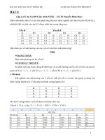
ACF and PACF:
In order to test the stationarity of the time series, let’s run the Augmented DickeyFuller Test using the adf.test function.
First set the hypothesis test:


The null hypothesis H0: that the time series is non stationary



The alternative hypothesis HA: that the time series is stationary

7


Where the p-value is less than 5%, we strong evidence against the null hypothesis, so
we reject the null hypothesis. In this case, if the test results which is >0.05 therefore
we accept the null hypothesis that the time series is non stationary.
A stationary time series has the conditions that the mean, variance and covariance are
not functions of time. In order to fit arima models, the time series is required to be
stationary. We will use two methods to test the stationarity.
Another way to test for stationarity is to use autocorrelation. We will use
autocorrelation function acf and partial autocorrelation function pacf. These functions
plot the correlation between a series and its lags ie previous observations with a 95%

confidence interval in blue. If the autocorrelation crosses the dashed blue line, it means
that specific lag is significantly correlated with current series.
Autocorrelation Function (ACF) and Partial Autocorrelation Function (PACF) The
ACF and PACF are used to figure out the order of AR, MA, and ARMA models. The
ACF and PACF plots can be obtained from the original data, as well as from the
residuals of a model. On the original data, these plots can help detect any
autoregressive or moving average terms that may be significant in the time series.
When applied to the residuals, these plots can detect any remaining autocorrelation in
the model. This also provides insight into whether additional AR or MA terms need
to be included in the model. Similarly, they can detect any seasonal behaviour that
must be accounted for in the model.

ARIMA MODEL:
We know that we need to address two issues before we test stationary series. One, we
need to remove unequal variances. We do this using log of the series. Two, we need
to address the trend component. We do this by taking difference of the series. Now,
let’s test the resultant series.

8


Differencing is the commonly used technique to remove non-stationarity. This
differencing is called as the Integration part in AR(I)MA. Now, we have three
parameters
p represents for AR
d represents for I
q represents for MA
An auto regressive (AR(p)) component is referring to the use of past values in the
regression equation for the series Y. The auto-regressive parameter p specifies the
number of lags used in the model.

The d represents the degree of differencing in the integrated (I(d)) component.
Differencing a series involves simply subtracting its current and previous values d
times.
A moving average (MA(q)) component represents the error of the model as a linear
combination of previous error terms et. The order q determines the number of terms
to include in the model
Seasonality can easily be incorporated in the ARIMA model directly.
ARIMA stands for Auto Regression Integrated Moving Average. It is specified by
three ordered parameters (p,d,q):


p is the order of the autoregressive model (number of time lags)



d is the degree of differencing (number of times the data have had past values
subtracted)



q is the order of moving average model.

Due the fact that our times series exhibits seasonality, we will use actually a model
called SARIMA, that is, as name suggest, a seasonality ARIMA. We write SARIMA
as ARIMA(p,d,q)(P, D, Q)m:
9




p — the number of autoregressive



d — degree of differencing



q — the number of moving average terms



m — refers to the number of periods in each season



(P, D, Q)— represents the (p,d,q) for the seasonal part of the time series

Use the auto.arima function to fit the best model and coefficients, given the default
parameters including seasonality as TRUE.

It is frequently used to predict demand, such as when estimating future demand for
atmospheric CO2. This is so that managers have solid parameters to follow when
making judgments about how to limit pollution. Based on historical data, ARIMA
models can also be used to forecast how much CO2 our environment will contain in
the future.

Fit model:
Model fitting is a measure of how well a machine learning model generalizes to
similar data to that on which it was trained. A model that is well-fitted produces more

accurate outcomes. A model that is overfitted matches the data too closely. A model
that is underfitted doesn’t match closely enough.

A machine learning model's model fitting is a gauge of how well it generalizes to data
that is comparable to the data it was trained on. We are able to use machine learning
algorithms every day to make predictions and classify data because they can
generalize a model to fresh data. When a model is given unknown inputs, a good
model fit is one that closely approximates the outcome of an unknown input. The
process of fitting a model involves changing its parameters in order to increase its
accuracy. A machine learning method is applied to data for which the target variable
is known ("labeled" data) in order to produce a machine learning model. In our case
10


we refuse to use linear model because it does not capture the seasonality and additive
effects over time.

Section 3: Application
Load libraries and data:
The first thing to do is to load the first data set we will use. This data set contains
observations on the concentration of carbon dioxide (CO2) in the atmosphere made at
Mauna Loa from 1958 to 2020. This is an in-built data set in R so can be loaded via
the data function
library(ggfortify)
library(tseries)
library(forecast)

Import data:
ts2 <- read.csv("C:/Users/HP/Downloads/co2_mm_mlo.csv")

Data cleaning:

We clarify the data by using sum(is.na(ts2)) to find not
available data and na.omit to delete those data in table

sum(is.na(ts2))
na.omit(ts2)->ts1

Invert data to time series model:

Dấu $ dùng để trích biến
val từ data ts1.

co=ts(ts1$val,start = 1958 , end = 2020, frequency = 12)
summary(co)
ylab <- expression(CO[2] ~ (ppm))
autoplot(co) + labs(x ="Year", y = ylab, title="Mauna Loa CO2
(PPM) from 1958 to 2020")

11


- autoplot is a generic function to visualize various data object
- tries to give better default graphics and customized choices for
each data type, quick and convenient to explore your genomic
data

Figure 1: Time series of the data

According to the graph, the variance of CO2 concentration remains relatively

constant throughout the survey time period, resulting in it being an additive model.
An additive model is the one in which the time series is the sum of trend,
seasonality, and remainder.

Time series decomposition
decomposeCO2 <- decompose(co,"additive")
autoplot(decomposeCO2)
"decompose" to Decompose a time series into seasonal, trend and irregular
components using moving averages. Deals with additive or multiplicative
seasonal component.
In this case, we use additive model.

additive model: Y[t]=T[t]+S[t]+e[t]
Y(t) is the concentration of co2 at time t,
T(t) is the trend component at time t,
S(t) is the seasonal component at time t,
e(t) is the random error component at time t.

12


Figure 2: Time series decomposition

Based on the graph of the trend, it can be seen that there is an upward trend
presented. The fact that the diagram of seasonality displays the same frequency and
magnitude solidifies the appropriacy of the additive model. Besides, since the mean
value of remainder is at 0, there is little to no correlation between the random values
confirming the fitness of the model.

Test stationary:

We know that we need to address two issues before we test stationary series.
One, we need to remove unequal variances. We do this using log of the series.
Two, we need to address the trend component. We do this by taking difference of
the series. Now, let’s test the resultant series.

We divide into 2 methods
ADF test:
adf.test(co)

In this case, as per the test results above, the p-value is 0.99 >0.05 therefore we accept
the null hypothesis that the time series is non stationary.

13


Autocorrelation (ACF & PACF)
autoplot(acf(co,plot=FALSE))+ labs(title="Correlogram of CO2
from 1958 to 2020")
autoplot(pacf(co,plot=FALSE))+ labs(title="Correlogram of CO2
from 1958 to 2020")

Figure 3: ACF diagram with trend and seasonality

Figure 4: PACF diagram with trend and seasonality

14


From the figure of ACF and PACF show that the lags of the ACF series decrease

gradually whilst the lags of the PACF series dies out quickly. Hence, the series is
most likely non-stationary.

Remove trend and seasonal effect

diff(log(co)): remove trend and seasonal effect to create a
new test.

ADF test:
adf.test(diff(log(co)), alternative="stationary", k=0)

In this case, as per the test results above, the p-value is 0.01<0.05 therefore we reject
the null hypothesis that the time series is non stationary.

ACF & PACF test:
autoplot(acf(diff(log(co)),plot=FALSE))+
labs(title="Correlogram of CO2 from 1958 to 2020")
autoplot(pacf(diff(log(co)),plot=FALSE))+
labs(title="Correlogram of CO2 from 1958 to 2020")

15


Figure 5: ACF diagram without trend and seasonality

Figure 6: PACF diagram without trend and seasonality

After remove the trend and the seasonality, the two graphs have a few significant
lags that die out quickly, which is prove that the series is most likely stationary.

16


geom_smooth() adds a trend line over an existing plot.
method="lm" use liner regression model to specific a trend line

FIT model:
Since there is an upwards trend we will look at a linear model first for comparison.
We plot the raw dataset with a linear model.
autoplot(co) + geom_smooth(method="lm")+ labs(x ="Year", y =
ylab, title="Mauna Loa CO2 (PPM) from 1958 to 2020")

Figure 7: Linear regression model of the data

This may not be best model to fit as it doesn’t capture the seasonality and additive
effects over time.
Use the auto.arima function to fit the best model and coefficients, given the
default parameters including seasonality as TRUE.

ARIMA Model
arimaCO2 <- auto.arima(co)
arimaCO2

17


SARIMA is the best model for forcasting

ggtsdiag : plot time series
diagnostic.

ggtsdiag(arimaCO2)

Figure 8: Diagrams of different analysis of residuals for model selection

The above figure shows the ACF of the residuals for a model. The “lag” (time span
between observations) is shown along the horizontal, and the autocorrelation is on the
vertical. The lines indicated bounds for statistical significance. The residual plots
appear to be centered around 0 as noise, with no pattern. Ljung-Box test show a pvalue pretty high so the SARIMA model is a fairly good fit.
Vẽ hình thành 1 cột và 2 dòng.

par(mfrow=c(1,2))
hist(residuals(arimaCO2),
xlab='CO2 PPM')

main='Mauna

qqnorm(residuals(arimaCO2))
18

Loa

CO2

Monthly',


The second graph (Normal Q-Q) plots
normalized error values, allowing to test the
assumption about the normal distribution of

residuals.

qqline(residuals(arimaCO2))

have a bell-shaped
=> normal
distribution.

Figure 9: Histogram and Q-Q Plot of the residuals

Remainder data is normally distributed so we can conclude that this model is best
fitted for our data since all of the correlation between the data in the dataset have been
considered.

Based on the graph, we see that the residuals are mostly concentrated
on the normal distribution
expected line, so the normal distribution of the residuals is assumed to
be satisfied.

Forecast
forecastCO2 <- forecast(arimaCO2, level = c(95), h = 24)
autoplot(forecastCO2)
level of confidence: 95%
h: forecast horizon periods
in months.

19


Figure 10: Time series forecast

Based on what the forecast showed, a continual increase in CO2 concentration will be
witnessed during the next two years.

Section 4: Conclusion
Thanks to the forecast, it is obvious that the concentration of CO 2 on Earth will
continue to rise without the any human-related activity. If we do not stop producing
additional CO2, its concentration will soon reach a level that is lethal for human
survival. Therefore, it is our mission to cut down on the amount of CO 2 from our
industries that is released into the environment so as not to worsen the current
situation. The reduction of CO2 can be accomplished by changing from fossil fuels to
green alternative energy like solar or wind energy. By refraining from using gas-based
cars and turning to electricity-based cars, we can also help to reduce the emission of
CO2. Besides, the transition from commuting by cars to bikes also helps as bikes do
not emit CO2 and they also help to improve humans’ health. Governments play a vital
role in this campaign as they are the only ones capable of passing laws that force
businesses to stop releasing too much CO2 by making them treat their polluted air
waste before it is let loose into the environment.

20


Section 5: R Code
library(ggfortify)
library(tseries)
library(forecast)
ts2 <- read.csv("C:/Users/HP/Downloads/co2_mm_mlo.csv")
sum(is.na(ts2))
na.omit(ts2)->ts1
co=ts(ts1$val,start = 1958 , end = 2020, frequency = 12)

summary(co)
ylab <- expression(CO[2] ~ (ppm))
autoplot(co) + labs(x ="Year", y = ylab, title="Mauna Loa CO2
(PPM) from 1958 to 2020")
decomposeCO2 <- decompose(co,"additive")
autoplot(decomposeCO2)
adf.test(co)
autoplot(acf(co,plot=FALSE))+ labs(title="Correlogram of CO2 from
1958 to 2020")
autoplot(pacf(co,plot=FALSE))+ labs(title="Correlogram of CO2 from
1958 to 2020")
adf.test(diff(log(co)), alternative="stationary", k=0)
autoplot(acf(diff(log(co)),plot=FALSE))+ labs(title="Correlogram
of CO2 from 1958 to 2020")
autoplot(pacf(diff(log(co)),plot=FALSE))+ labs(title="Correlogram
of CO2 from 1958 to 2020")
autoplot(co) + geom_smooth(method="lm")+ labs(x ="Year", y = ylab,
title="Mauna Loa CO2 (PPM) from 1958 to 2020")
arimaCO2 <- auto.arima(co)
arimaCO2
ggtsdiag(arimaCO2)
par(mfrow=c(1,2))
hist(residuals(arimaCO2), main='Mauna Loa CO2 Monthly', xlab='CO2
PPM')
qqnorm(residuals(arimaCO2))
qqline(residuals(arimaCO2))
forecastCO2 <- forecast(arimaCO2, level = c(95), h = 24)
autoplot(forecastCO2)

21

Reference
1. Time series analysis methods: />2. RPubs – Time series analysis of atmospheric CO2 levels at Mauna Loa:
/>3. A comprehensive guide to time series analysis:
/>4. How to choose the right TS model for your prediction:
/>5. Time series analysis: Definition, types, techniques and when it is used:
/>
22