CFA curriculum 2023 level 1 volume 1: QUANTITATIVE METHODS
Bạn đang xem bản rút gọn của tài liệu. Xem và tải ngay bản đầy đủ của tài liệu tại đây (6.87 MB, 512 trang )
© CFA Institute. For candidate use only. Not for distribution.
QUANTITATIVE
METHODS
CFA® Program Curriculum
2023 • LEVEL 1 • VOLUME 1
© CFA Institute. For candidate use only. Not for distribution.
©2022 by CFA Institute. All rights reserved. This copyright covers material written
expressly for this volume by the editor/s as well as the compilation itself. It does
not cover the individual selections herein that first appeared elsewhere. Permission
to reprint these has been obtained by CFA Institute for this edition only. Further
reproductions by any means, electronic or mechanical, including photocopying and
recording, or by any information storage or retrieval systems, must be arranged with
the individual copyright holders noted.
CFA®, Chartered Financial Analyst®, AIMR-PPS®, and GIPS® are just a few of the
trademarks owned by CFA Institute. To view a list of CFA Institute trademarks and the
Guide for Use of CFA Institute Marks, please visit our website at www.cfainstitute.org.
This publication is designed to provide accurate and authoritative information
in regard to the subject matter covered. It is sold with the understanding that the
publisher is not engaged in rendering legal, accounting, or other professional service.
If legal advice or other expert assistance is required, the services of a competent professional should be sought.
All trademarks, service marks, registered trademarks, and registered service marks
are the property of their respective owners and are used herein for identification
purposes only.
ISBN 978-1-950157-96-9 (paper)
ISBN 978-1-953337-23-8 (ebook)
2022
© CFA Institute. For candidate use only. Not for distribution.
CONTENTS
How to Use the CFA Program Curriculum
Errata
Designing Your Personal Study Program
CFA Institute Learning Ecosystem (LES)
Feedback
ix
ix
ix
x
x
Learning Module 1
The Time Value of Money
Introduction
Interest Rates
Future Value of a Single Cash Flow
Non-Annual Compounding (Future Value)
Continuous Compounding
Stated and Effective Rates
A Series of Cash Flows
Equal Cash Flows—Ordinary Annuity
Unequal Cash Flows
Present Value of a Single Cash Flow
Non-Annual Compounding (Present Value)
Present Value of a Series of Equal and Unequal Cash Flows
The Present Value of a Series of Equal Cash Flows
The Present Value of a Series of Unequal Cash Flows
Present Value of a Perpetuity
Present Values Indexed at Times Other than t = 0
Solving for Interest Rates, Growth Rates, and Number of Periods
Solving for Interest Rates and Growth Rates
Solving for the Number of Periods
Solving for Size of Annuity Payments
Present and Future Value Equivalence and the Additivity Principle
The Cash Flow Additivity Principle
Summary
Practice Problems
Solutions
3
3
4
6
10
12
14
15
15
16
17
19
21
21
25
26
27
28
29
31
32
36
38
39
40
45
Learning Module 2
Organizing, Visualizing, and Describing Data
Introduction
Data Types
Numerical versus Categorical Data
Cross-Sectional versus Time-Series versus Panel Data
Structured versus Unstructured Data
Data Summarization
Organizing Data for Quantitative Analysis
Summarizing Data Using Frequency Distributions
Summarizing Data Using a Contingency Table
59
59
60
61
63
64
68
68
71
77
Quantitative Methods
indicates an optional segment
iv
© CFA Institute. For candidate use only. Not for distribution.
Contents
Data Visualization
Histogram and Frequency Polygon
Bar Chart
Tree-Map
Word Cloud
Line Chart
Scatter Plot
Heat Map
Guide to Selecting among Visualization Types
Measures of Central Tendency
The Arithmetic Mean
The Median
The Mode
Other Concepts of Mean
Quantiles
Quartiles, Quintiles, Deciles, and Percentiles
Quantiles in Investment Practice
Measures of Dispersion
The Range
The Mean Absolute Deviation
Sample Variance and Sample Standard Deviation
Downside Deviation and Coefficient of Variation
Coefficient of Variation
The Shape of the Distributions
The Shape of the Distributions: Kurtosis
Correlation between Two Variables
Properties of Correlation
Limitations of Correlation Analysis
Summary
Practice Problems
Solutions
82
82
84
87
88
90
92
96
98
100
101
105
106
107
116
117
122
123
123
124
125
128
131
133
136
139
140
143
146
151
164
Learning Module 3
Probability Concepts
Probability Concepts and Odds Ratios
Probability, Expected Value, and Variance
Conditional and Joint Probability
Expected Value and Variance
Portfolio Expected Return and Variance of Return
Covariance Given a Joint Probability Function
Bayes' Formula
Bayes’ Formula
Principles of Counting
Summary
References
Practice Problems
Solutions
173
174
174
179
191
197
202
206
206
212
218
220
221
228
Learning Module 4
Common Probability Distributions
Discrete Random Variables
235
236
indicates an optional segment
Contents
© CFA Institute. For candidate use only. Not for distribution.
v
Discrete Random Variables
Discrete and Continuous Uniform Distribution
Continuous Uniform Distribution
Binomial Distribution
Normal Distribution
The Normal Distribution
Probabilities Using the Normal Distribution
Standardizing a Random Variable
Probabilities Using the Standard Normal Distribution
Applications of the Normal Distribution
Lognormal Distribution and Continuous Compounding
The Lognormal Distribution
Continuously Compounded Rates of Return
Student’s t-, Chi-Square, and F-Distributions
Student’s t-Distribution
Chi-Square and F-Distribution
Monte Carlo Simulation
Summary
Practice Problems
Solutions
237
241
243
246
254
254
258
260
260
262
266
266
269
272
272
274
279
285
288
296
Learning Module 5
Sampling and Estimation
Introduction
Sampling Methods
Simple Random Sampling
Stratified Random Sampling
Cluster Sampling
Non-Probability Sampling
Sampling from Different Distributions
The Central Limit Theorem and Distribution of the Sample Mean
The Central Limit Theorem
Standard Error of the Sample Mean
Point Estimates of the Population Mean
Point Estimators
Confidence Intervals for the Population Mean and Sample Size Selection
Selection of Sample Size
Resampling
Sampling Related Biases
Data Snooping Bias
Sample Selection Bias
Look-Ahead Bias
Time-Period Bias
Summary
Practice Problems
Solutions
303
304
304
305
306
308
309
313
315
315
317
320
320
324
330
332
335
336
337
339
340
341
344
349
Learning Module 6
Hypothesis Testing
Introduction
Why Hypothesis Testing?
353
354
354
indicates an optional segment
vi
Learning Module 7
© CFA Institute. For candidate use only. Not for distribution.
Contents
Implications from a Sampling Distribution
The Process of Hypothesis Testing
Stating the Hypotheses
Two-Sided vs. One-Sided Hypotheses
Selecting the Appropriate Hypotheses
Identify the Appropriate Test Statistic
Test Statistics
Identifying the Distribution of the Test Statistic
Specify the Level of Significance
State the Decision Rule
Determining Critical Values
Decision Rules and Confidence Intervals
Collect the Data and Calculate the Test Statistic
Make a Decision
Make a Statistical Decision
Make an Economic Decision
Statistically Significant but Not Economically Significant?
The Role of p-Values
Multiple Tests and Significance Interpretation
Tests Concerning a Single Mean
Test Concerning Differences between Means with Independent Samples
Test Concerning Differences between Means with Dependent Samples
Testing Concerning Tests of Variances
Tests of a Single Variance
Test Concerning the Equality of Two Variances (F-Test)
Parametric vs. Nonparametric Tests
Uses of Nonparametric Tests
Nonparametric Inference: Summary
Tests Concerning Correlation
Parametric Test of a Correlation
Tests Concerning Correlation: The Spearman Rank Correlation
Coefficient
Test of Independence Using Contingency Table Data
Summary
References
Practice Problems
Solutions
355
356
357
357
358
359
359
360
360
362
363
364
365
366
366
366
366
367
370
373
377
379
383
383
387
392
393
393
394
395
Introduction to Linear Regression
Simple Linear Regression
Estimating the Parameters of a Simple Linear Regression
The Basics of Simple Linear Regression
Estimating the Regression Line
Interpreting the Regression Coefficients
Cross-Sectional vs. Time-Series Regressions
Assumptions of the Simple Linear Regression Model
Assumption 1: Linearity
Assumption 2: Homoskedasticity
Assumption 3: Independence
429
429
432
432
433
436
437
440
440
442
444
indicates an optional segment
397
399
404
407
408
419
Contents
© CFA Institute. For candidate use only. Not for distribution.
vii
Assumption 4: Normality
Analysis of Variance
Breaking down the Sum of Squares Total into Its Components
Measures of Goodness of Fit
ANOVA and Standard Error of Estimate in Simple Linear Regression
Hypothesis Testing of Linear Regression Coefficients
Hypothesis Tests of the Slope Coefficient
Hypothesis Tests of the Intercept
Hypothesis Tests of Slope When Independent Variable Is an
Indicator Variable
Test of Hypotheses: Level of Significance and p-Values
Prediction Using Simple Linear Regression and Prediction Intervals
Functional Forms for Simple Linear Regression
The Log-Lin Model
The Lin-Log Model
The Log-Log Model
Selecting the Correct Functional Form
Summary
Practice Problems
Solutions
445
447
448
449
450
453
453
456
Appendices
493
indicates an optional segment
457
459
460
464
465
466
468
469
471
474
488
© CFA Institute. For candidate use only. Not for distribution.
© CFA Institute. For candidate use only. Not for distribution.
How to Use the CFA
Program Curriculum
The CFA® Program exams measure your mastery of the core knowledge, skills, and
abilities required to succeed as an investment professional. These core competencies
are the basis for the Candidate Body of Knowledge (CBOK™). The CBOK consists of
four components:
■
A broad outline that lists the major CFA Program topic areas (www.
cfainstitute.org/programs/cfa/curriculum/cbok)
■
Topic area weights that indicate the relative exam weightings of the top-level
topic areas (www.cfainstitute.org/programs/cfa/curriculum)
■
Learning outcome statements (LOS) that advise candidates about the specific knowledge, skills, and abilities they should acquire from curriculum
content covering a topic area: LOS are provided in candidate study sessions and at the beginning of each block of related content and the specific
lesson that covers them. We encourage you to review the information about
the LOS on our website (www.cfainstitute.org/programs/cfa/curriculum/
study-sessions), including the descriptions of LOS “command words” on the
candidate resources page at www.cfainstitute.org.
■
The CFA Program curriculum that candidates receive upon exam
registration
Therefore, the key to your success on the CFA exams is studying and understanding
the CBOK. You can learn more about the CBOK on our website: www.cfainstitute.
org/programs/cfa/curriculum/cbok.
The entire curriculum, including the practice questions, is the basis for all exam
questions and is selected or developed specifically to teach the knowledge, skills, and
abilities reflected in the CBOK.
ERRATA
The curriculum development process is rigorous and includes multiple rounds of
reviews by content experts. Despite our efforts to produce a curriculum that is free
of errors, there are instances where we must make corrections. Curriculum errata are
periodically updated and posted by exam level and test date online on the Curriculum
Errata webpage (www.cfainstitute.org/en/programs/submit-errata). If you believe you
have found an error in the curriculum, you can submit your concerns through our
curriculum errata reporting process found at the bottom of the Curriculum Errata
webpage.
DESIGNING YOUR PERSONAL STUDY PROGRAM
An orderly, systematic approach to exam preparation is critical. You should dedicate
a consistent block of time every week to reading and studying. Review the LOS both
before and after you study curriculum content to ensure that you have mastered the
ix
x
© CFA Institute. For candidate use only. Not for distribution.
How to Use the CFA Program Curriculum
applicable content and can demonstrate the knowledge, skills, and abilities described
by the LOS and the assigned reading. Use the LOS self-check to track your progress
and highlight areas of weakness for later review.
Successful candidates report an average of more than 300 hours preparing for each
exam. Your preparation time will vary based on your prior education and experience,
and you will likely spend more time on some study sessions than on others.
CFA INSTITUTE LEARNING ECOSYSTEM (LES)
Your exam registration fee includes access to the CFA Program Learning Ecosystem
(LES). This digital learning platform provides access, even offline, to all of the curriculum content and practice questions and is organized as a series of short online lessons
with associated practice questions. This tool is your one-stop location for all study
materials, including practice questions and mock exams, and the primary method by
which CFA Institute delivers your curriculum experience. The LES offers candidates
additional practice questions to test their knowledge, and some questions in the LES
provide a unique interactive experience.
FEEDBACK
Please send any comments or feedback to , and we will review
your suggestions carefully.
© CFA Institute. For candidate use only. Not for distribution.
Quantitative Methods
© CFA Institute. For candidate use only. Not for distribution.
© CFA Institute. For candidate use only. Not for distribution.
LEARNING MODULE
1
The Time Value of Money
by Richard A. DeFusco, PhD, CFA, Dennis W. McLeavey, DBA, CFA, Jerald
E. Pinto, PhD, CFA, and David E. Runkle, PhD, CFA.
Richard A. DeFusco, PhD, CFA, is at the University of Nebraska-Lincoln (USA). Dennis W.
McLeavey, DBA, CFA, is at the University of Rhode Island (USA). Jerald E. Pinto, PhD,
CFA, is at CFA Institute (USA). David E. Runkle, PhD, CFA, is at Jacobs Levy Equity
Management (USA).
LEARNING OUTCOME
Mastery
The candidate should be able to:
interpret interest rates as required rates of return, discount rates, or
opportunity costs
explain an interest rate as the sum of a real risk-free rate and
premiums that compensate investors for bearing distinct types of
risk
calculate and interpret the future value (FV) and present value (PV)
of a single sum of money, an ordinary annuity, an annuity due, a
perpetuity (PV only), and a series of unequal cash flows
demonstrate the use of a time line in modeling and solving time
value of money problems
calculate the solution for time value of money problems with
different frequencies of compounding
calculate and interpret the effective annual rate, given the stated
annual interest rate and the frequency of compounding
INTRODUCTION
As individuals, we often face decisions that involve saving money for a future use, or
borrowing money for current consumption. We then need to determine the amount
we need to invest, if we are saving, or the cost of borrowing, if we are shopping for
a loan. As investment analysts, much of our work also involves evaluating transactions with present and future cash flows. When we place a value on any security, for
example, we are attempting to determine the worth of a stream of future cash flows.
To carry out all the above tasks accurately, we must understand the mathematics of
time value of money problems. Money has time value in that individuals value a given
amount of money more highly the earlier it is received. Therefore, a smaller amount
1
4
Learning Module 1
© CFA Institute. For candidate use only. Not for distribution.
The Time Value of Money
of money now may be equivalent in value to a larger amount received at a future date.
The time value of money as a topic in investment mathematics deals with equivalence
relationships between cash flows with different dates. Mastery of time value of money
concepts and techniques is essential for investment analysts.
The reading1 is organized as follows: Section 2 introduces some terminology used
throughout the reading and supplies some economic intuition for the variables we will
discuss. Section 3 tackles the problem of determining the worth at a future point in
time of an amount invested today. Section 4 addresses the future worth of a series of
cash flows. These two sections provide the tools for calculating the equivalent value at
a future date of a single cash flow or series of cash flows. Sections 5 and 6 discuss the
equivalent value today of a single future cash flow and a series of future cash flows,
respectively. In Section 7, we explore how to determine other quantities of interest
in time value of money problems.
2
INTEREST RATES
interpret interest rates as required rates of return, discount rates, or
opportunity costs
explain an interest rate as the sum of a real risk-free rate and
premiums that compensate investors for bearing distinct types of
risk
In this reading, we will continually refer to interest rates. In some cases, we assume
a particular value for the interest rate; in other cases, the interest rate will be the
unknown quantity we seek to determine. Before turning to the mechanics of time
value of money problems, we must illustrate the underlying economic concepts. In
this section, we briefly explain the meaning and interpretation of interest rates.
Time value of money concerns equivalence relationships between cash flows
occurring on different dates. The idea of equivalence relationships is relatively simple.
Consider the following exchange: You pay $10,000 today and in return receive $9,500
today. Would you accept this arrangement? Not likely. But what if you received the
$9,500 today and paid the $10,000 one year from now? Can these amounts be considered
equivalent? Possibly, because a payment of $10,000 a year from now would probably
be worth less to you than a payment of $10,000 today. It would be fair, therefore,
to discount the $10,000 received in one year; that is, to cut its value based on how
much time passes before the money is paid. An interest rate, denoted r, is a rate of
return that reflects the relationship between differently dated cash flows. If $9,500
today and $10,000 in one year are equivalent in value, then $10,000 − $9,500 = $500
is the required compensation for receiving $10,000 in one year rather than now. The
interest rate—the required compensation stated as a rate of return—is $500/$9,500
= 0.0526 or 5.26 percent.
Interest rates can be thought of in three ways. First, they can be considered required
rates of return—that is, the minimum rate of return an investor must receive in order
to accept the investment. Second, interest rates can be considered discount rates. In
the example above, 5.26 percent is that rate at which we discounted the $10,000 future
amount to find its value today. Thus, we use the terms “interest rate” and “discount
rate” almost interchangeably. Third, interest rates can be considered opportunity costs.
1 Examples in this reading and other readings in quantitative methods at Level I were updated in 2018 by
Professor Sanjiv Sabherwal of the University of Texas, Arlington.
Interest Rates
© CFA Institute. For candidate use only. Not for distribution.
An opportunity cost is the value that investors forgo by choosing a particular course
of action. In the example, if the party who supplied $9,500 had instead decided to
spend it today, he would have forgone earning 5.26 percent on the money. So we can
view 5.26 percent as the opportunity cost of current consumption.
Economics tells us that interest rates are set in the marketplace by the forces of supply and demand, where investors are suppliers of funds and borrowers are demanders
of funds. Taking the perspective of investors in analyzing market-determined interest
rates, we can view an interest rate r as being composed of a real risk-free interest rate
plus a set of four premiums that are required returns or compensation for bearing
distinct types of risk:
r = Real risk-free interest rate + Inflation premium + Default risk premium +
Liquidity premium + Maturity premium
■
The real risk-free interest rate is the single-period interest rate for a completely risk-free security if no inflation were expected. In economic theory,
the real risk-free rate reflects the time preferences of individuals for current
versus future real consumption.
■
The inflation premium compensates investors for expected inflation and
reflects the average inflation rate expected over the maturity of the debt.
Inflation reduces the purchasing power of a unit of currency—the amount
of goods and services one can buy with it. The sum of the real risk-free
interest rate and the inflation premium is the nominal risk-free interest
rate.2 Many countries have governmental short-term debt whose interest
rate can be considered to represent the nominal risk-free interest rate in that
country. The interest rate on a 90-day US Treasury bill (T-bill), for example,
represents the nominal risk-free interest rate over that time horizon.3 US
T-bills can be bought and sold in large quantities with minimal transaction
costs and are backed by the full faith and credit of the US government.
■
The default risk premium compensates investors for the possibility that the
borrower will fail to make a promised payment at the contracted time and in
the contracted amount.
■
The liquidity premium compensates investors for the risk of loss relative
to an investment’s fair value if the investment needs to be converted to cash
quickly. US T-bills, for example, do not bear a liquidity premium because
large amounts can be bought and sold without affecting their market price.
Many bonds of small issuers, by contrast, trade infrequently after they are
issued; the interest rate on such bonds includes a liquidity premium reflecting the relatively high costs (including the impact on price) of selling a
position.
■
The maturity premium compensates investors for the increased sensitivity
of the market value of debt to a change in market interest rates as maturity
is extended, in general (holding all else equal). The difference between the
2 Technically, 1 plus the nominal rate equals the product of 1 plus the real rate and 1 plus the inflation rate.
As a quick approximation, however, the nominal rate is equal to the real rate plus an inflation premium.
In this discussion we focus on approximate additive relationships to highlight the underlying concepts.
3 Other developed countries issue securities similar to US Treasury bills. The French government issues
BTFs or negotiable fixed-rate discount Treasury bills (Bons du Trésor àtaux fixe et à intérêts précomptés)
with maturities of up to one year. The Japanese government issues a short-term Treasury bill with maturities of 6 and 12 months. The German government issues at discount both Treasury financing paper
(Finanzierungsschätze des Bundes or, for short, Schätze) and Treasury discount paper (Bubills) with
maturities up to 24 months. In the United Kingdom, the British government issues gilt-edged Treasury
bills with maturities ranging from 1 to 364 days. The Canadian government bond market is closely related
to the US market; Canadian Treasury bills have maturities of 3, 6, and 12 months.
5
6
Learning Module 1
© CFA Institute. For candidate use only. Not for distribution.
The Time Value of Money
interest rate on longer-maturity, liquid Treasury debt and that on short-term
Treasury debt reflects a positive maturity premium for the longer-term debt
(and possibly different inflation premiums as well).
Using this insight into the economic meaning of interest rates, we now turn to a
discussion of solving time value of money problems, starting with the future value
of a single cash flow.
3
FUTURE VALUE OF A SINGLE CASH FLOW
calculate and interpret the future value (FV) and present value (PV)
of a single sum of money, an ordinary annuity, an annuity due, a
perpetuity (PV only), and a series of unequal cash flows
demonstrate the use of a time line in modeling and solving time
value of money problems
In this section, we introduce time value associated with a single cash flow or lump-sum
investment. We describe the relationship between an initial investment or present
value (PV), which earns a rate of return (the interest rate per period) denoted as r,
and its future value (FV), which will be received N years or periods from today.
The following example illustrates this concept. Suppose you invest $100 (PV =
$100) in an interest-bearing bank account paying 5 percent annually. At the end of
the first year, you will have the $100 plus the interest earned, 0.05 × $100 = $5, for a
total of $105. To formalize this one-period example, we define the following terms:
PV = present value of the investment
FVN = future value of the investment N periods from today
r = rate of interest per period
For N = 1, the expression for the future value of amount PV is
FV1 = PV(1 + r)
(1)
For this example, we calculate the future value one year from today as FV1 = $100(1.05)
= $105.
Now suppose you decide to invest the initial $100 for two years with interest
earned and credited to your account annually (annual compounding). At the end of
the first year (the beginning of the second year), your account will have $105, which
you will leave in the bank for another year. Thus, with a beginning amount of $105
(PV = $105), the amount at the end of the second year will be $105(1.05) = $110.25.
Note that the $5.25 interest earned during the second year is 5 percent of the amount
invested at the beginning of Year 2.
Another way to understand this example is to note that the amount invested at
the beginning of Year 2 is composed of the original $100 that you invested plus the
$5 interest earned during the first year. During the second year, the original principal
again earns interest, as does the interest that was earned during Year 1. You can see
how the original investment grows:
Original investment
$100.00
Interest for the first year ($100 × 0.05)
5.00
Interest for the second year based on original investment ($100 × 0.05)
5.00
© CFA Institute. For candidate use only. Not for distribution.
Future Value of a Single Cash Flow
Interest for the second year based on interest earned in the first year (0.05 ×
$5.00 interest on interest)
Total
0.25
$110.25
The $5 interest that you earned each period on the $100 original investment is known
as simple interest (the interest rate times the principal). Principal is the amount of
funds originally invested. During the two-year period, you earn $10 of simple interest.
The extra $0.25 that you have at the end of Year 2 is the interest you earned on the
Year 1 interest of $5 that you reinvested.
The interest earned on interest provides the first glimpse of the phenomenon
known as compounding. Although the interest earned on the initial investment is
important, for a given interest rate it is fixed in size from period to period. The compounded interest earned on reinvested interest is a far more powerful force because,
for a given interest rate, it grows in size each period. The importance of compounding
increases with the magnitude of the interest rate. For example, $100 invested today
would be worth about $13,150 after 100 years if compounded annually at 5 percent,
but worth more than $20 million if compounded annually over the same time period
at a rate of 13 percent.
To verify the $20 million figure, we need a general formula to handle compounding
for any number of periods. The following general formula relates the present value of
an initial investment to its future value after N periods:
FVN = PV(1 + r)N
(2)
where r is the stated interest rate per period and N is the number of compounding
periods. In the bank example, FV2 = $100(1 + 0.05)2 = $110.25. In the 13 percent
investment example, FV100 = $100(1.13)100 = $20,316,287.42.
The most important point to remember about using the future value equation is
that the stated interest rate, r, and the number of compounding periods, N, must be
compatible. Both variables must be defined in the same time units. For example, if
N is stated in months, then r should be the one-month interest rate, unannualized.
A time line helps us to keep track of the compatibility of time units and the interest
rate per time period. In the time line, we use the time index t to represent a point in
time a stated number of periods from today. Thus the present value is the amount
available for investment today, indexed as t = 0. We can now refer to a time N periods
from today as t = N. The time line in Exhibit 1 shows this relationship.
Exhibit 1: The Relationship between an Initial Investment, PV, and Its Future
Value, FV
0
PV
1
2
3
...
N–1
N
FVN = PV(1 + r)N
In Exhibit 1, we have positioned the initial investment, PV, at t = 0. Using Equation
2, we move the present value, PV, forward to t = N by the factor (1 + r)N. This factor
is called a future value factor. We denote the future value on the time line as FV and
7
8
Learning Module 1
© CFA Institute. For candidate use only. Not for distribution.
The Time Value of Money
position it at t = N. Suppose the future value is to be received exactly 10 periods from
today’s date (N = 10). The present value, PV, and the future value, FV, are separated
in time through the factor (1 + r)10.
The fact that the present value and the future value are separated in time has
important consequences:
■
We can add amounts of money only if they are indexed at the same point in
time.
■
For a given interest rate, the future value increases with the number of
periods.
■
For a given number of periods, the future value increases with the interest
rate.
To better understand these concepts, consider three examples that illustrate how
to apply the future value formula.
EXAMPLE 1
The Future Value of a Lump Sum with Interim Cash
Reinvested at the Same Rate
1. You are the lucky winner of your state’s lottery of $5 million after taxes.
You invest your winnings in a five-year certificate of deposit (CD) at a local
financial institution. The CD promises to pay 7 percent per year compounded annually. This institution also lets you reinvest the interest at that rate for
the duration of the CD. How much will you have at the end of five years if
your money remains invested at 7 percent for five years with no withdrawals?
Solution:
To solve this problem, compute the future value of the $5 million investment
using the following values in Equation 2:
PV = $5, 000, 000
r = 7 % = 0.07
N = 5
N
F
)
V N =
PV (1 + r
= $5,000,000 ( 1.07) 5
= $5,000,000 ( 1.402552)
= $7,012,758.65
At the end of five years, you will have $7,012,758.65 if your money remains
invested at 7 percent with no withdrawals.
In this and most examples in this reading, note that the factors are reported at six
decimal places but the calculations may actually reflect greater precision. For example, the reported 1.402552 has been rounded up from 1.40255173 (the calculation is
actually carried out with more than eight decimal places of precision by the calculator
or spreadsheet). Our final result reflects the higher number of decimal places carried
by the calculator or spreadsheet.4
4 We could also solve time value of money problems using tables of interest rate factors. Solutions using
tabled values of interest rate factors are generally less accurate than solutions obtained using calculators
or spreadsheets, so practitioners prefer calculators or spreadsheets.
© CFA Institute. For candidate use only. Not for distribution.
Future Value of a Single Cash Flow
EXAMPLE 2
The Future Value of a Lump Sum with No Interim Cash
1. An institution offers you the following terms for a contract: For an investment of ¥2,500,000, the institution promises to pay you a lump sum six
years from now at an 8 percent annual interest rate. What future amount
can you expect?
Solution:
Use the following data in Equation 2 to find the future value:
PV = ¥2, 500, 000
r = 8 % = 0.08
N = 6
N
F
V N =
PV (1 + r)
= ¥2, 500, 000 ( 1.08) 6
= ¥2, 500, 000 ( 1.586874)
= ¥3, 967, 186
You can expect to receive ¥3,967,186 six years from now.
Our third example is a more complicated future value problem that illustrates the
importance of keeping track of actual calendar time.
EXAMPLE 3
The Future Value of a Lump Sum
1. A pension fund manager estimates that his corporate sponsor will make
a $10 million contribution five years from now. The rate of return on plan
assets has been estimated at 9 percent per year. The pension fund manager
wants to calculate the future value of this contribution 15 years from now,
which is the date at which the funds will be distributed to retirees. What is
that future value?
Solution:
By positioning the initial investment, PV, at t = 5, we can calculate the future
value of the contribution using the following data in Equation 2:
PV = $10 million
r = 9 % = 0.09
N = 10
N
F
V N =
PV (1 + r
)
= $10,000,000 ( 1.09) 10
= $10,000,000 ( 2.367364)
= $23,673,636.75
This problem looks much like the previous two, but it differs in one important respect: its timing. From the standpoint of today (t = 0), the future
amount of $23,673,636.75 is 15 years into the future. Although the future
value is 10 years from its present value, the present value of $10 million will
not be received for another five years.
9
10
Learning Module 1
© CFA Institute. For candidate use only. Not for distribution.
The Time Value of Money
Exhibit 2: The Future Value of a Lump Sum, Initial Investment Not at
t=0
As Exhibit 2 shows, we have followed the convention of indexing today
as t = 0 and indexing subsequent times by adding 1 for each period. The
additional contribution of $10 million is to be received in five years, so it is
indexed as t = 5 and appears as such in the figure. The future value of the
investment in 10 years is then indexed at t = 15; that is, 10 years following
the receipt of the $10 million contribution at t = 5. Time lines like this one
can be extremely useful when dealing with more-complicated problems,
especially those involving more than one cash flow.
In a later section of this reading, we will discuss how to calculate the value today
of the $10 million to be received five years from now. For the moment, we can use
Equation 2. Suppose the pension fund manager in Example 3 above were to receive
$6,499,313.86 today from the corporate sponsor. How much will that sum be worth
at the end of five years? How much will it be worth at the end of 15 years?
PV = $6,499,313.86
r = 9 % = 0.09
N = 5
N
F
V N =
PV (1 + r)
= $6,499,313.86 ( 1.09) 5
= $6,499,313.86 ( 1.538624)
= $10,000,000 at the five-year mark
and
PV = $6,499,313.86
r = 9 % = 0.09
N = 15
N
F
V N =
PV (1 + r)
= $6,499,313.86 ( 1.09) 15
= $6,499,313.86 ( 3.642482)
= $23,673,636.74 at the 15-year mark
These results show that today’s present value of about $6.5 million becomes $10
million after five years and $23.67 million after 15 years.
4
NON-ANNUAL COMPOUNDING (FUTURE VALUE)
calculate the solution for time value of money problems with
different frequencies of compounding
© CFA Institute. For candidate use only. Not for distribution.
Non-Annual Compounding (Future Value)
In this section, we examine investments paying interest more than once a year. For
instance, many banks offer a monthly interest rate that compounds 12 times a year.
In such an arrangement, they pay interest on interest every month. Rather than quote
the periodic monthly interest rate, financial institutions often quote an annual interest
rate that we refer to as the stated annual interest rate or quoted interest rate. We
denote the stated annual interest rate by rs. For instance, your bank might state that
a particular CD pays 8 percent compounded monthly. The stated annual interest rate
equals the monthly interest rate multiplied by 12. In this example, the monthly interest
rate is 0.08/12 = 0.0067 or 0.67 percent.5 This rate is strictly a quoting convention
because (1 + 0.0067)12 = 1.083, not 1.08; the term (1 + rs) is not meant to be a future
value factor when compounding is more frequent than annual.
With more than one compounding period per year, the future value formula can
be expressed as
rs mN
m )
FV N = PV (1 + _
(3)
where rs is the stated annual interest rate, m is the number of compounding
periods per year, and N now stands for the number of years. Note the compatibility
here between the interest rate used, rs/m, and the number of compounding periods,
mN. The periodic rate, rs/m, is the stated annual interest rate divided by the number
of compounding periods per year. The number of compounding periods, mN, is the
number of compounding periods in one year multiplied by the number of years. The
periodic rate, rs/m, and the number of compounding periods, mN, must be compatible.
EXAMPLE 4
The Future Value of a Lump Sum with Quarterly
Compounding
1. Continuing with the CD example, suppose your bank offers you a CD with
a two-year maturity, a stated annual interest rate of 8 percent compounded
quarterly, and a feature allowing reinvestment of the interest at the same
interest rate. You decide to invest $10,000. What will the CD be worth at
maturity?
Solution:
Compute the future value with Equation 3 as follows:
PV = $10,000
r s = 8 % = 0.08
m = 4
rs / m = 0.08 / 4 = 0.02
N = 2
mN
4 (2) = 8 interest periods
=
rs mN
FV N = PV (1 + _
m )
= $10,000 ( 1.02) 8
= $10,000 ( 1.171659)
= $11,716.59
At maturity, the CD will be worth $11,716.59.
5 To avoid rounding errors when using a financial calculator, divide 8 by 12 and then press the %i key,
rather than simply entering 0.67 for %i, so we have (1 + 0.08/12)12 = 1.083000.
11
12
Learning Module 1
© CFA Institute. For candidate use only. Not for distribution.
The Time Value of Money
The future value formula in Equation 3 does not differ from the one in Equation 2.
Simply keep in mind that the interest rate to use is the rate per period and the exponent is the number of interest, or compounding, periods.
EXAMPLE 5
The Future Value of a Lump Sum with Monthly
Compounding
1. An Australian bank offers to pay you 6 percent compounded monthly. You
decide to invest A$1 million for one year. What is the future value of your
investment if interest payments are reinvested at 6 percent?
Solution:
Use Equation 3 to find the future value of the one-year investment as follows:
PV = A$1,000,000
r s = 6 % = 0.06
m = 12
rs / m = 0.06 / 12 = 0.0050
N = 1
mN
(1) = 12 interest periods
12
=
rs mN
FV N = PV (1 + _
m )
= A$1,000,000 ( 1.005) 12
= A$1,000,000 ( 1.061678)
= A$1,061,677.81
If you had been paid 6 percent with annual compounding, the future
amount would be only A$1,000,000(1.06) = A$1,060,000 instead of
A$1,061,677.81 with monthly compounding.
5
CONTINUOUS COMPOUNDING
calculate and interpret the effective annual rate, given the stated
annual interest rate and the frequency of compounding
calculate the solution for time value of money problems with
different frequencies of compounding
The preceding discussion on compounding periods illustrates discrete compounding,
which credits interest after a discrete amount of time has elapsed. If the number of
compounding periods per year becomes infinite, then interest is said to compound
continuously. If we want to use the future value formula with continuous compounding, we need to find the limiting value of the future value factor for m → ∞ (infinitely
many compounding periods per year) in Equation 3. The expression for the future
value of a sum in N years with continuous compounding is
FV N = PV e rs N
(4)
© CFA Institute. For candidate use only. Not for distribution.
Continuous Compounding
13
The term e rs N is the transcendental number e ≈ 2.7182818 raised to the power rsN.
Most financial calculators have the function ex.
EXAMPLE 6
The Future Value of a Lump Sum with Continuous
Compounding
Suppose a $10,000 investment will earn 8 percent compounded continuously
for two years. We can compute the future value with Equation 4 as follows:
PV = $10,000
rs = 8 % = 0.08
N = 2
r N
F
PV e s
V N =
= $10,000 e 0.08 ( 2)
= $10,000 ( 1.173511)
= $11,735.11
With the same interest rate but using continuous compounding, the $10,000
investment will grow to $11,735.11 in two years, compared with $11,716.59
using quarterly compounding as shown in Example 4.
Exhibit 3 shows how a stated annual interest rate of 8 percent generates different
ending dollar amounts with annual, semiannual, quarterly, monthly, daily, and continuous compounding for an initial investment of $1 (carried out to six decimal places).
As Exhibit 3 shows, all six cases have the same stated annual interest rate of 8
percent; they have different ending dollar amounts, however, because of differences
in the frequency of compounding. With annual compounding, the ending amount
is $1.08. More frequent compounding results in larger ending amounts. The ending
dollar amount with continuous compounding is the maximum amount that can be
earned with a stated annual rate of 8 percent.
Exhibit 3: The Effect of Compounding Frequency on Future Value
Frequency
Annual
rs/m
mN
8%/1 = 8%
1×1=1
Semiannual
8%/2 = 4%
2×1=2
Quarterly
8%/4 = 2%
4×1=4
Monthly
8%/12 = 0.6667%
12 × 1 = 12
Daily
Continuous
8%/365 = 0.0219%
365 × 1 = 365
Future Value of $1
$1.00(1.08)
$1.00(1.04)2
$1.00(1.02)4
$1.00(1.006667)12
$1.00(1.000219)365
$1.00e0.08(1)
Exhibit 3 also shows that a $1 investment earning 8.16 percent compounded annually
grows to the same future value at the end of one year as a $1 investment earning 8
percent compounded semiannually. This result leads us to a distinction between the
stated annual interest rate and the effective annual rate (EAR).6 For an 8 percent
stated annual interest rate with semiannual compounding, the EAR is 8.16 percent.
6 Among the terms used for the effective annual return on interest-bearing bank deposits are annual
percentage yield (APY) in the United States and equivalent annual rate (EAR) in the United Kingdom.
By contrast, the annual percentage rate (APR) measures the cost of borrowing expressed as a yearly
=
$1.08
=
$1.081600
=
$1.082432
=
$1.083000
=
$1.083278
=
$1.083287
14
Learning Module 1
© CFA Institute. For candidate use only. Not for distribution.
The Time Value of Money
Stated and Effective Rates
The stated annual interest rate does not give a future value directly, so we need a formula for the EAR. With an annual interest rate of 8 percent compounded semiannually,
we receive a periodic rate of 4 percent. During the course of a year, an investment of
$1 would grow to $1(1.04)2 = $1.0816, as illustrated in Exhibit 3. The interest earned
on the $1 investment is $0.0816 and represents an effective annual rate of interest of
8.16 percent. The effective annual rate is calculated as follows:
EAR = (1 + Periodic interest rate)m – 1
(5)
The periodic interest rate is the stated annual interest rate divided by m, where m is
the number of compounding periods in one year. Using our previous example, we can
solve for EAR as follows: (1.04)2 − 1 = 8.16 percent.
The concept of EAR extends to continuous compounding. Suppose we have a rate
of 8 percent compounded continuously. We can find the EAR in the same way as above
by finding the appropriate future value factor. In this case, a $1 investment would
grow to $1e0.08(1.0) = $1.0833. The interest earned for one year represents an effective
annual rate of 8.33 percent and is larger than the 8.16 percent EAR with semiannual
compounding because interest is compounded more frequently. With continuous
compounding, we can solve for the effective annual rate as follows:
EAR = e rs − 1
(6)
We can reverse the formulas for EAR with discrete and continuous compounding to
find a periodic rate that corresponds to a particular effective annual rate. Suppose we
want to find the appropriate periodic rate for a given effective annual rate of 8.16 percent with semiannual compounding. We can use Equation 5 to find the periodic rate:
0.0816 = ( 1 + Periodic rate) 2 − 1
1.0816 = ( 1 + Periodic rate) 2
1.0816) 1/2 − 1 = Periodic rate
(
( 1.04) − 1 = Periodic rate
4% = Periodic rate
To calculate the continuously compounded rate (the stated annual interest rate with
continuous compounding) corresponding to an effective annual rate of 8.33 percent,
we find the interest rate that satisfies Equation 6:
0.0833 = e rs − 1
1.0833 = e rs
To solve this equation, we take the natural logarithm of both sides. (Recall that the
natural log of e r s is ln e r s = r s .) Therefore, ln 1.0833 = rs, resulting in rs = 8 percent. We
see that a stated annual rate of 8 percent with continuous compounding is equivalent
to an EAR of 8.33 percent.
rate. In the United States, the APR is calculated as a periodic rate times the number of payment periods
per year and, as a result, some writers use APR as a general synonym for the stated annual interest rate.
Nevertheless, APR is a term with legal connotations; its calculation follows regulatory standards that vary
internationally. Therefore, “stated annual interest rate” is the preferred general term for an annual interest
rate that does not account for compounding within the year.
A Series of Cash Flows
© CFA Institute. For candidate use only. Not for distribution.
15
6
A SERIES OF CASH FLOWS
calculate and interpret the future value (FV) and present value (PV)
of a single sum of money, an ordinary annuity, an annuity due, a
perpetuity (PV only), and a series of unequal cash flows
demonstrate the use of a time line in modeling and solving time
value of money problems
In this section, we consider series of cash flows, both even and uneven. We begin
with a list of terms commonly used when valuing cash flows that are distributed over
many time periods.
■
An annuity is a finite set of level sequential cash flows.
■
An ordinary annuity has a first cash flow that occurs one period from now
(indexed at t = 1).
■
An annuity due has a first cash flow that occurs immediately (indexed at t
= 0).
■
A perpetuity is a perpetual annuity, or a set of level never-ending sequential cash flows, with the first cash flow occurring one period from now.
Equal Cash Flows—Ordinary Annuity
Consider an ordinary annuity paying 5 percent annually. Suppose we have five separate deposits of $1,000 occurring at equally spaced intervals of one year, with the first
payment occurring at t = 1. Our goal is to find the future value of this ordinary annuity
after the last deposit at t = 5. The increment in the time counter is one year, so the
last payment occurs five years from now. As the time line in Exhibit 4 shows, we find
the future value of each $1,000 deposit as of t = 5 with Equation 2, FVN = PV(1 + r)N.
The arrows in Exhibit 4 extend from the payment date to t = 5. For instance, the first
$1,000 deposit made at t = 1 will compound over four periods. Using Equation 2, we
find that the future value of the first deposit at t = 5 is $1,000(1.05)4 = $1,215.51. We
calculate the future value of all other payments in a similar fashion. (Note that we
are finding the future value at t = 5, so the last payment does not earn any interest.)
With all values now at t = 5, we can add the future values to arrive at the future value
of the annuity. This amount is $5,525.63.
Exhibit 4: The Future Value of a Five-Year Ordinary Annuity
0
|
1
$1,000
|
2
$1,000
|
3
$1,000
|
4
$1,000
|
5
$1,000(1.05)4
$1,000(1.05)3
$1,000(1.05)2
$1,000(1.05)1
=
=
=
=
$1,215.506250
$1,157.625000
$1,102.500000
$1,050.000000
$1,000(1.05)0 = $1,000.000000
Sum at t = 5
$5,525.63