2809 f 8585171167157815952 04 23 015
Bạn đang xem bản rút gọn của tài liệu. Xem và tải ngay bản đầy đủ của tài liệu tại đây (1.01 MB, 9 trang )
JST: Smart Systems and Devices
Volume 33, Issue 2, May 2023, 026-034
Discrete-Time Backstepping Sliding Mode Control
for a 2-DOF PAM-Based Exoskeleton
Van-Vuong Dinh1,2, Van-Long Nguyen1, Kim-Chien Hoang1,
Minh-Duc Duong1, Quy-Thinh Dao1*
Hanoi University of Science and Technology, Ha Noi, Vietnam.
2
Hanoi College of High Technology, Ha Noi, Vietnam.
*
Corresponding author email:
1
Abstract
This study aims to propose a discrete-time backstepping sliding mode control technique (BSMC) for regulating
a pneumatic artificial muscle (PAM)-based exoskeleton used in rehabilitating human lower extremities. The
PAM system is challenging to control due to its high nonlinearity, parameter uncertainty, and significant delay
resulting from using compressed air. A backstepping control method is a recursive approach that
systematically designs control laws for nonlinear and complicated systems. This technique ensures stable and
robust system control, even in uncertain circumstances. Furthermore, the backstepping controller can handle
high-order systems and guarantee high-precision tracking of a desired trajectory. The incorporation of sliding
mode control is aimed at enhancing the performance of the robot PAM system by reducing chattering and
reaching time. The algorithm employs Lyapunov functions and sliding surfaces to design the control signal for
operating the system. The study concludes with experimental scenarios demonstrating the effectiveness of
the proposed approach.
Keywords: Pneumatic artificial muscle, backstepping, sliding mode control
1. Introduction 1
the objects in practice are nonlinear, we often linearize
these objects to simplify the control. However, the
system will only work well within certain limits. The
PAMs system mentioned in this paper is nonlinear,
with considerable latency and uncertain parameters.
Such systems always attract great attention from
researchers. The problem with these systems of PAMs
is determining a nonlinear mathematical model that
leads to errors in estimating the system's parameters.
As a result, PAM-based systems have a lot of unknown
disturbances. Multiple control methods have been
offered to solve the problems of pneumatic muscle
actuator control. The Proportional-Integral-Derivative
(PID) controller and its enhanced versions are the most
researched. For example, a nonlinear PID-based
controller [5, 6] enhances the correction of nonlinear
hysteresis phenomena and increases robustness. The
Fuzzy PID controllers [7, 8] are offered to increase the
trajectory tracking performance. The neural network
PID controllers [9, 10] are trained to provide the
optimum value for various set frequencies and load
conditions. Most of the mentioned controllers have
decent performance and specific advantages and
disadvantages. However, the PID controller is also
unsuitable for objects with high nonlinearity and delay
characteristics, so it does not guarantee the
optimization and stability of the system.
Rehabilitation robots are often expensive due to
their high manufacturing cost, mainly because electric
motors power them [1, 2]. However, a growing interest
is in developing low-cost robots that can operate
efficiently. In recent years, pneumatic artificial
muscles (PAMs) have emerged as one of the most
promising actuators for simulating human movements.
PAMs are lightweight, low-cost, and easy to
manufacture. The power-to-weight ratio is also a
significant concern. Therefore, researchers are
increasingly studying PAMs and their applications in
rehabilitation robots, medical devices for motor
function recovery, and control programs to enhance
human safety while working with robots. The
cylindrical braided muscle [3], known as McKibben’s
in the 1950s, is currently the most popular type of
artificial pneumatic muscle. Besides the mentioned
advantage [4] PAMs have several limitations,
including high nonlinearity, uncertain parameters, and
high impact delay. Therefore, modeling and control
pneumatic artificial muscles have recently become an
interesting topic for researchers.
Regarding the design of control algorithms for
rehabilitation robots using pneumatic artificial
muscles, we have two main control algorithms: Linear
and nonlinear control. For linear control, since most of
ISSN: 2734-9373
/>Received: March 1, 2023; accepted: April 7, 2023
26
JST: Smart Systems and Devices
Volume 33, Issue 2, May 2023, 026-034
This paper proposes the BSMC algorithm as one
of the most widely used approaches for highly
nonlinear systems. BSMC is a distinct nonlinear
control technique integrating the backstepping control
design approach and sliding mode control controller.
The Backstepping control law, developed in the 1990s
by Petar V. Kokotovic and other researchers [11], is
designed to develop stabilizing controls for a particular
category of nonlinear dynamical systems. It is a
nonlinear control approach with the primary advantage
of handling complex nonlinear systems and
disturbances, making it applicable to various
applications.
muscles, installed in an antagonistic configuration
with one another through a pulley, drive each joint.
Specifically, a 1-inch-diameter McKibben artificial
muscle was utilized, which, like human muscles, has a
maximum contraction of 30% of muscle length. The
proportional control valve ITV2030-212S-X26 from
sliding mode control (SMC) is employed for PAMs'
pressure adjustment. The rotation angles are measured
using a WDD35D4 rotary potentiometer coaxially
mounted to two couplings.
In addition, loadcell sensors are installed on the
single-ended muscle tubes to measure the pulling force
of each muscle. The control algorithm is implemented
using the NI Myrio platform, developed by National
Instrument. The NI Myrio control computer acquires
voltage signals from various sources, including
loadcells and potentiometers. The control program is
then developed and compiled using Labview software
and downloaded to NI Myrio to create a closed-loop
control system.
Moreover, backstepping can be utilized to design
robust controllers insensitive to modeling errors and
uncertainties while providing better tracking and
disturbance rejection performance compared to other
control techniques. These nonlinear dynamical
systems are composed of subsystems that extend from
a primary subsystem, which can be stabilized using
another method. The recursive structure of the system
enables the designer to commence the design process
at the stable subsystem and sequentially stabilize each
outer subsystem by developing new controllers using
a "backing out" approach. In this study, we aim to
stabilize the control variables, such as acceleration,
velocity, and the joint angle corresponding to the
robot. The algorithm will rely on the selection of
Lyapunov functions and sliding surfaces to design the
control signal that will stabilize the system according
to Lyapunov [12, 13]. By incorporating backstepping
and sliding mode control, the proposed algorithm
provides more effectiveness than the conventional
sliding control algorithm [14-16]. To summarize, this
paper makes the following contributions:
-
Development of a discrete-time backstepping
sliding mode control for a pneumatic artificial
muscle-based exoskeleton;
-
The proposed controller's effectiveness is
demonstrated through various experimental
scenarios to verify its suitability for robotic
rehabilitation systems utilizing a pneumatic
artificial muscle actuator.
Fig. 1. The experimental model of a robot system using
a pneumatic artificial muscle actuator.
The paper's structure is as follows: Section 2
outlines the experimental platform, equipment, and a
mathematical model of a PAM-based exoskeleton.
Section 3 describes the design of the proposed
controller. Section 4 demonstrates the experimental
results. Lastly, section 5 summarizes the research and
discusses possible future work.
2. Robotic System Modeling
(a)
Fig. 1 illustrates a robot system that utilizes a
pneumatic artificial muscle actuator. This system is
designed for lower extremity rehabilitation and
features a hip and knee joint affixed to a flat surface to
facilitate movement. A pair of pneumatic artificial
(b)
Fig. 2. (a) The schematic diagram of PAM. (b) The
three-element model of PAM.
27
JST: Smart Systems and Devices
Volume 33, Issue 2, May 2023, 026-034
To model the PAM robot system, we refer to
Reynolds’s three-element model [17] of a single PAM
as shown in Fig. 2. Accordingly, the model can be
represented by the equation:
M
y + B( P) y + K ( P) y =F ( P) − Mg
)
K ( P=
=
B
P
(
)
with
P)
B( =
F ( P=
)
Let the input pressure of the anterior muscles
( Pa ) and posterior muscles ( Pp ) are:
Pa= P0 + ∆P + PAP
(2)
Pp= P0 − ∆P
The initial different pressure PAP is added so the
robot is upright at the initial position.
(1)
K 0 + K1 P
B0i + B1i P
(inflation)
The contraction of the anterior muscle ( ya ) and
B0 j + B1 j P (deflation)
posterior muscle ( y p ) can be determined using the
F0 + F1 P
following equations:
where y is the amount of the PAM contraction. K ( P)
B( P) , F ( P) are the model's spring, damping, and
contractile elements. P is the input pressure of the
PAM. The parameter value B will depend on when
the PAM contracts Bi or deflates B j .
y0 − Rθ
y=
a
(3)
y0 + Rθ
y=
p
where R is the radius of the joint, y0 is the muscle's
initial contraction, and θ is the joint's rotation angle.
Based on the report [18], the torque generated can
be expressed as follows:
The robotic system is designed to operate as
follows: Each joint of the robotic orthosis is actuated
by two PAMs in an antagonistic setup. In this setup,
each joint’s anterior and posterior muscles have been
initially provided with similar pressure P0 . Therefore
they have the same length. We create rotation by
increasing the pressure on one side of the muscle while
the pressure on the other decreases ∆P . Therefore,
∆P is the control variable. A detailed description of
the structure of the robot system is shown in Fig. 3.
T = ( Fa − K a ya − Ba y a )
(4)
− Fp − K p y p − B p y p R
where Fa , K a , and Ba depend on the input pressure
of anterior muscle and Fp , K p , and B p depend on the
(
)
input pressure of posterior muscle according to to (1).
Fig. 3. The structure of hip and knee muscles with an antagonistic configuration
28
JST: Smart Systems and Devices
Volume 33, Issue 2, May 2023, 026-034
exists in the system, the state-space model of the
dynamic system (9) can be represented as follows:
Thus,
T = F1 PAP + 2 K 0 Rθ − K1 ( PAP ya + P0 ya − P0 y p )
x1 (t ) = θ(t )
x (t ) = x (t )
1
2
x 2 (t ) = f (x1 (t ), x 2 (t ), ψ (t ))
+ ( ∆λψ (t ) + λ ) u(t )
− ( B0 a + B1a P0 + B1a PAP ) y a + ( B0 p + B1 p P0 ) y p R
+ [ 2 F1 − B1a y a + B1 p y p R∆P
(5)
(
f (t ) = H −1 −V ′θ − J ′
where λ = H −1c4
u(t ) = ∆P
Substituting ya , y p from (3) into (5). The torque
T created by anterior and posterior PAMs to the joint
can be obtained as follows:
=
T c1 + c2θ + c3θ + c4 ∆P
(6)
c1 = F1 PAP R
2
c2 =( 2 K 0 + 2 K1 P0 + K1 PAP ) R
c = B + B + B + B P + B P R 2
( 0a 0 p ) 0 1a AP
0p
3 0a
2
c4 = 2 F1 R − ( B1a − B1 p ) R θ
+ Vθ + J =
Hθ
T
(7)
y (k + 1)= y (k ) + Ts y1 (k )
= y1 (k ) + Ts y 2 (k )
y1 (k + 1)
y 2 (k ) = f ( y1 (k ), y 2 (t ), ψ (k ) )
+ ( ∆λψ (k ) + λ ) u(k )
y (k + 1)= y (k ) + Ts y1 (k )
= y1 (k ) + Ts y 2 (k )
y1 (k + 1)
y =
2 (k ) ζ(k ) + λu(k )
θ= H −1 ( −V ′θ − J ′ ) + ( H −1c 4 ) ΔP
(9)
(12)
3. Controller Design
This section introduces the proposed BSMC
technique, which has two primary goals: Maintaining
system stability and regulating the mechanical rotation
angle y ( k ) to track a reference signal y* ( k ) , that
mimics the actual motion of the human foot. Fig. 4
depicts the control block diagram of the BSMC
approach. The backstepping control method
decomposes the second-order system model into
smaller subsystems. At each stage, the virtual control
law y1 ( k ) and y2 ( k ) for the corresponding
From (6) and (7), we have:
(8)
(11)
By setting ζ(k ) f (y1 (k ), y 2 (t ), ψ (k )) + ∆λψ (k )u(k ) ,
=
the model (11) becomes:
θ h
Here, θ = represents the coordinates of the
θ k
Th
robot joints and T = represents the torque matrix
Tk
generated by the effects of the PAMs on the robot's
joints. Additionally H , V , J denote the inertia,
viscous moment and radial force matrices, and the
gravity torque matrix.
+ Vθ + J =
Hθ
c1 + c 2 θ + c3θ + c 4 ΔP
)
Assume y ( k ) , y 1 ( k ) , y 2 ( k ) are the muscle's
matrix, velocity, and acceleration, respectively. The
discrete-time model for the dynamic system of PAM
can be obtained from the following:
where
From the torque of the PAM-based actuator in
equation (6), we consider the dynamic behavior of the
PAM-based 2-DOF robot as the following equation:
(10)
Thus
subsystems are developed using the discrete-time
Lyapunov stability theorem. With strictly Lyapunov
stability functions, the recursive algorithm assures the
proposed BSMC strategy's internal dynamic stability.
In step 3, the sliding-mode control approach
guarantees that the system state trajectory reaches the
sliding surface and that the system disturbance current
tracking error reduces to zero.
V=′ V − c3
with
J ′ =J − c 2 θ − c1
0
c
c2 h 0
c1h
where c1 = , c 2 =
, c 3 = 3h
0 c2 k
c1k
0 c3k
0
∆Ph
c
c4 = 4 h
∆P , h , and k denote the
, ∆P =
0
c
4k
k
hip and knee joints, respectively. By including the term
ψ (t ) , which denotes the unknown disturbance that
STEP 1: Aims to establish a tracking error vector
that measures the difference between the controlled
rotation angle y ( k ) and the reference signal y* ( k ) :
e=
(k ) y (k ) − y* (k )
29
(13)
JST: Smart Systems and Devices
Volume 33, Issue 2, May 2023, 026-034
Fig. 4. Block diagram of the controller.
Select the initial Lyapunov function candidate as:
V1 (k ) = e(k )
We can define the first virtual control law vector
y2* ( k ) in step 1 as follows, with y2 ( k ) representing
(14)
2
the initial virtual control law vector:
Hence, the variation of V1 ( k ) can be obtained as:
y2* (k ) =
∆V1 (k )= V1 (k + 1) − V1 (k )
2
= y (k + 1) − y* (k + 1) − e(k ) 2
= y (k ) + Ts e1 (k ) + Ts y1* (k )
2
∆V2 (k=
) Ts y2 (k ) − Ts y2* (k )
− (1 − Ts2 )e1 (k ) 2 − e(k ) 2
− y* (k + 1) − e(k ) 2
The initial virtual control law vector is denoted as
y1 (k ) can be expressed as the first vector in the
=
sequence of virtual control laws, starting with y1* (k )
in step 1, which is defined as follows:
y* (k + 1) − y (k )
Ts
Substituting (16) into (15) yields:
− (1 − T )e1 (k ) − e(k )
2
STEP 3: At this stage, a sliding-mode control
approach is applied after completing the two steps in
the backstepping design process. The sliding-surface
vector is formulated as:
s (k ) =e2 (k ) + α e1 (k ) + β e(k )
V=
e (k ) + V1 (k )
2 (k )
The derivative of V3 ( k ) can be obtained as:
e1 (k + 1)= y1 (k + 1) − y1* (k + 1)
(19)
2
2
∆V3=
( k ) s ( k ) − s ( k − 1) + ∆V2 ( k )
= s ( k ) [ e2 ( k ) + α e1 ( k ) + β e( k ) ]
The derivative of V2 (k ) can be calculated as:
− s ( k − 1) + [Ts e2 ( k ) ]
2
2
k ) e1 (k + 1) − e1 (k ) + ∆V1 (k )
∆V2 (=
2
(24)
V3 (k ) = s (k − 1) 2 + V2 (k )
Using (13), it is possible to derive the error vector
for e2 as:
= y1 (k ) + Ts y2 (k ) − y1* (k + 1)
(23)
where α and β are positive constants, a third
candidate for the Lyapunov function is defined as:
(18)
( y1 (k ) + Ts y2 (k ) − y (k + 1) )
2
zero.
2
1
=
(22)
2
s
equals 0. Therefore, the next stage is determining the
vector of e2 ( k ) that leads to convergence towards
(16)
2
*
1
[Ts e2 (k )]
2
By examining (22), it becomes evident that
∆V2 ( k ) will become negative definite if e2 ( k )
∆V1 (k=
) Ts y1 (k ) − Ts y1* (k ) − e(k ) 2
(17)
= Ts2 e1 (k ) 2 − e(k ) 2
STEP 2: To guarantee the convergence of the
vector e1 (k ) to zero, we can choose the second
Lyapunov function as:
2
(21)
Substituting (21) into (20), we have:
(15)
2
y1* (k ) =
y1* (k + 1) − y1 (k )
Ts
2
−(1 − Ts2 )e1 ( k ) 2 − e( k ) 2
(20)
− (1 − Ts2 )e1 (k ) 2 − e(k ) 2
30
(25)
JST: Smart Systems and Devices
Volume 33, Issue 2, May 2023, 026-034
algorithms on the rehabilitation robot to evaluate the
efficacy of the control methodology presented. The hip
and knee angle reference trajectories will be adjusted
for each subject by modifying the gait data profile in
[19], with the hip and knee flexion/extension angles
ranging from -13.5º to 16.5º and -40º to 0º,
respectively. The control algorithm will be developed
using the Lab-VIEW/MyRIO toolkit and then
integrated into the MyRIO 1900 controller with a 5 ms
sampling time. We will test multiple scenarios to
evaluate and improve the practicality of the control
method. Specifically, the experiment will be
conducted at frequencies of 0.2 Hz or 0.5 Hz under two
scenarios: with and without a load. The parameters for
both the BSMC and SMC controllers will be finetuned and summarized in Table 1.
The calculated deviation e2 (k ) is:
e=
y2 ( k ) − y * 2 ( k )
2 (k )
(26)
=
− y *2 ( k ) − ζ ( k ) − λ u ( k )
In the proposed BSMC method, it is assumed that
the control law vector has the following structure:
u (k ) = λ −1 − y*2 (k ) − ζ (k ) − ρ sign ( s (k ) )
− ( 2 + γ ) e2 (k ) − α e1 (k ) − β e(k )
(27)
where γ is a positive number added to satisfy the
condition ∆V3 (k ) ≤ 0 in equation (29).
Subsequently, the derivative of V3 (k ) can be
represented as:
Table 1. Parameters of the BSMC and SMC controllers
∆V3 (k ) = s (k ) [ −γ e2 (k ) ] − ρ s (k ) sign ( s (k ) )
− s (k − 1) 2 + [Ts e2 (k ) ]
2
(28)
−(1 − Ts2 )e1 (k ) 2 − e(k ) 2
We can arrive at the following equation by
replacing (28) with (27):
γβ
∆V3 (k ) ≤ − s (k − 1) 2 − e(k ) + e2 (k )
2
2
2
s
γ 2β 2
α 2γ 2
− γ −
−
− Ts2 e2 (k ) 2
2
4
4(1 − Ts )
β
γ
0.025
0.1
1
0.5
0.025
0.1
ρ
BSMC
SMC
Both control strategies demonstrate effective
tracking performance in the first scenario without a
load. The joint angle signals of the robot tracked the
sample trajectory and achieved a steady state in less
1
cycle gait. However, the BSMC controller
than
4
outperforms the SMC controller with higher
performance and fewer errors, as demonstrated in
Fig. 5 and Fig. 6. Specifically, the SMC controller
exhibits an oscillation amplitude of about 3.8º for the
hip joint, while the BSMC controller's amplitude is
only about 1.4º and the deviation value fluctuates
around 0º. At 0.5 Hz, both control methods exhibit
reduced performance, but the BSMC controller is still
better at tracking the trajectory. The effectiveness of
the proposed controller is further demonstrated by the
root mean square error (RMSE) values, which are
3.46° and 2.11° for the hip and knee joints,
respectively, with the BSMC controller. In
comparison, the SMC controller produces RMSE
values of 3.89° and 2.68° for the same joints.
2
e (k )
−(1 − T ) e1 (k ) + αγ 2 2
2(1 − Ts )
α
Parameters
(29)
Equation (29) enables the selection of a set of
numbers α , β and γ that ensure the stability of the
Lyapunov function. Therefore, the proposed
backstepping sliding mode control guarantees the
system's stability.
4. Experimental Results
We will compare the control performance
achieved by implementing the BSMC and SMC
(b) Knee joint
(a) Hip joint
Fig. 5. Experimental results when tracking joint trajectory at 0.2 Hz without a load.
31
JST: Smart Systems and Devices
Volume 33, Issue 2, May 2023, 026-034
(a) Hip joint
(b) Knee joint
Fig. 6. Experimental results when tracking joint trajectory at 0.5 Hz without a load.
(a) Hip joint
(b) Knee joint
Fig. 7. Experimental results when tracking joint trajectory at 0.2 Hz with a load.
(a) Hip joint
(b) Knee joint
Fig. 8. Experimental results when tracking joint trajectory at 0.5 Hz with a load.
In the second scenario, where the rehabilitation
robot is subjected to external loads, the performance of
both controllers is decreased but still achieves
satisfactory accuracy. This scenario is significant
because rehabilitation robots typically encounter
external forces and loads in practical applications. The
load is placed at the position of the lower limb
exoskeleton robot, and the maximum impact force is
experienced when the leg is extended forward. We use
anthropometric data (described in Table 4 in the book
[20]) to determine the Rated Load to be applied
quantitatively. Since the study only focused on lower
extremity rehabilitation, the experiment will be
implemented with a variable load weighing 60 kg to 80
kg. The ratio of total leg weight to total body weight is
0.161. Each robot only controls one human leg, from
which we calculate the rated Load ranging from 48.3
N to 64.44 N. The author changed the Load as the Load
variable with the value from 0 N to 75.44 N.
Specifically, the explanation was also highlighted on
page 7 of the revised manuscript. As illustrated in Fig.
7, when observing the hip and knee angles with a
frequency of 0.2 Hz, the BSMC controller
demonstrates faster stabilization times. As the applied
force gradually increases to the maximum value, the
tracking error of BSMC stabilizes quickly, while SMC
spikes up quite high. When monitored at 0.2 Hz,
SMC's highest deviation of dynamic performance is
around 9.0º, whereas BSMC's figure is approximately
5.0º. At a frequency of 0.5 Hz, the BSMC controller
demonstrates a lower root mean square error (RMSE)
of 4.30° and 2.65° for the hip and knee joints,
respectively. In contrast, the SMC controller produces
RMSE values of 4.79° and 3.26° for the same joints.
Finally, the RMSE values of BSMC in Table 2 and
Table 2 demonstrate that it outperforms the SMC
controller.
32
JST: Smart Systems and Devices
Volume 33, Issue 2, May 2023, 026-034
Table 2. RMSE (°) of two controllers with hip joint
trajectory input.
Frequency
Without load
BSMC. The results in Table 4, Table 5, Table 6, and
Table 7 still show that the proposed BSMC controller
performs better. ISE integrates the square of the error
over time. Therefore, this index will increase sharply
when a large overshoot. This is most clearly
demonstrated when observing the knee angles with a
frequency of 0.5 Hz. While the ISE Index of the BSMC
controller is 57.20°, that of the SMC controller is up to
118.52°. IAE integrates the absolute error over time.
Therefore in the same case, the IAE index will be
smaller than ISE's. Specifically, the knee angles with a
frequency of 0.5 Hz is also observed. The ISE Index of
BSMC and SMC controller is 24.24° and 31.53°,
respectively.
Load
BSMC
SMC
BSMC
SMC
0.2 Hz
2.29
2.61
2.77
3.59
0.5 Hz
3.46
3.89
4.30
4.79
Table 3. RMSE (°) of two controllers with knee joint
trajectory input.
Frequency
Without load
Load
BSMC
SMC
BSMC
SMC
0.2 Hz
1.29
1.59
1.76
2.59
5. Conclusion
0.5 Hz
2.11
2.68
2.65
3.26
BSMC
SMC
BSMC
SMC
This paper proposes and applies the BSMC law to
the PAM-based robot to aid in the recovery of leg
muscle function for patients. The proposed controller
can manage the PAM robot's direction, velocity, and
acceleration based on desired references. The
backstepping law aims to mitigate chattering and
enhance the SMC method's tracking capabilities
during transient and steady-state operations. The
tracking precision of the BSMC controller is
evaluated, and the efficacy of the reaching law is
confirmed via various experimental scenarios. The
outcomes of the experiments indicate that the proposed
controller successfully addresses chattering issues and
delivers adequate tracking performance. The proposed
BSMC controller performs similarly with and without
load compared to SMC. For instance, when tracking a
knee joint with 0.2 Hz and 40º amplitude without load,
the BSMC controller's RMSEs reach 1.29º (3.23% of
amplitude), while the SMC controller achieves an
accuracy of 5.7%. In summary, the BSMC controller
reduces tracking errors and enhances performance
when tracking human gait patterns. The results suggest
the potential of this controller in rehabilitation robots.
However, the tracking error remains significant.
Additional control laws may be necessary to restore
patient function, such as using neural networks to
recognize human impedance and tracking errors.
0.2 Hz
18.78
20.35
22.45
29.43
Acknowledgments
0.5 Hz
30.43
34.27
32.63
38.10
This research was funded by Hanoi University of
Science and Technology (HUST) under project
number T2022-PC-002.
Table 4. ISE (°) of two controllers with hip joint
trajectory input.
Frequency
Without load
Load
BSMC
SMC
BSMC
SMC
0.2 Hz
78.39
112.58
103.36
140.58
0.5 Hz
104.06
135.62
125.71
154.87
Table 5. ISE (°) of two controllers with knee joint
trajectory input.
Frequency
Without load
Load
BSMC
SMC
BSMC
SMC
0.2 Hz
25.20
38.10
30.48
57.50
0.5 Hz
49.27
109.07
57.20
118.52
Table 6. IAE (°) of two controllers with hip joint
trajectory input.
Frequency
Without load
Load
Table 7. IAE (°) of two controllers with knee joint
trajectory input.
Frequency
0.2 Hz
Without load
References
Load
BSMC
SMC
BSMC
SMC
15.76
20.44
16.67
23.02
0.5 Hz
22.67
27.79
24.24
31.53
We calculated additional Integral Absolute Error
(IAE), Integral Squared Error (ISE) to contrast the
performance between SMC relatively and suggested
33
[1]
M. al Kouzbary, N. A. Abu Osman, A. K. Abdul
Wahab, Sensorless control system for assistive robotic
ankle-foot, Int J Adv Robot Syst, vol. 15, no. 3, May
2018,
/>
[2]
Z. Wang, L. Quan, and X. Liu, Sensorless SPMSM
position estimation using position estimation error
suppression control and EKF in wide speed range,
Math Probl Eng, vol. 2014, 2014,
/>
JST: Smart Systems and Devices
Volume 33, Issue 2, May 2023, 026-034
[3]
M. G. Antonelli, P. Beomonte Zobel, A. De Marcellis,
and E. Palange, Design and characterization of a
mckibben pneumatic muscle prototype with an
embedded capacitive length transducer, Machines, vol.
10, no. 12, Dec. 2022,
/>
[4]
S. M. Mirvakili, I. W. Hunter, Artificial muscles:
mechanisms, applications, and challenges, Advanced
Materials, vol. 30, no. 6. Wiley-VCH Verlag, Feb.
2018,
/>
[5]
J. Zhong, J. Fan, Y. Zhu, J. Zhao, and W. Zhai, One
nonlinear pid control to improve the control
performance of a manipulator actuated by a pneumatic
muscle
actuator,
Advances
in
Mechanical
Engineering, vol. 2014, 2014,
/>
[6]
G. Andrikopoulos, G. Nikolakopoulos and S. Manesis,
Non-linear control of Pneumatic Artificial Muscles,
21st Mediterranean Conference on Control and
Automation, Platanias, Greece, 2013, pp. 729-734,
10.1109/MED.2013.6608804.
[7]
J. Wu, J. Huang, Y. Wang, K. Xing and Q. Xu, Fuzzy
PID control of a wearable rehabilitation robotic hand
driven by pneumatic muscles, 2009 International
Symposium on Micro-NanoMechatronics and Human
Science, Nagoya, Japan, 2009, pp. 408-413,
10.1109/MHS.2009.5352012.
[8]
A. Koohestani and E. A. Moghadam, Controlling
muscle-joint system by functional electrical
stimulation using combination of PID and fuzzy
controller, APCBEE Procedia, vol. 7, pp. 156-162,
2013,
/>
[9]
[12] Y. Kim, T. H. Oh, T. Park, and J. M. Lee, Backstepping
control integrated with Lyapunov-based model
predictive control, J Process Control, vol. 73, pp. 137146, Jan. 2019,
/>[13] T. Liard, I. Ismaıla Balogoun, S. Marx, and F. Plestan,
Boundary sliding mode control of a system of linear
hyperbolic equations: a Lyapunov approach, 2021.
[Online]. Available:
/>05109821004908
[14] J. Wang, J. Liu, G. Zhang, and S. Guo, Periodic eventtriggered sliding mode control for lower limb
exoskeleton based on human-robot cooperation, ISA
Trans, vol. 123, pp. 87-97, Apr. 2022,
10.1016/j.isatra.2021.05.039.
[15] L. Melkou and M. Hamerlain, High Order
Homogeneous Sliding Mode Control for a Robot Arm
with Pneumatic Artificial Muscles, IECON 2019 - 45th
Annual Conference of the IEEE Industrial Electronics
Society, Lisbon, Portugal, 2019, pp. 394-399,
10.1109/IECON.2019.8927339.
[16] L. Zhao, H. Cheng, and T. Wang, Sliding mode control
for a two-joint coupling nonlinear system based on
extended state observer, ISA Trans, vol. 73, pp. 130140, Feb. 2018,
10.1016/j.isatra.2017.12.027.
[17] D. B. Reynolds, D. W. Repperger, C. A. Phillips, and
G. Bandry, Modeling the dynamic characteristics of
pneumatic muscle, Ann Biomed Eng, vol. 31, no. 3,
pp. 310-317, 2003,
10.1114/1.1554921.
[18] T. Y. Choi and J. J. Lee, Control of manipulator using
pneumatic muscles for enhanced safety, IEEE
Transactions on Industrial Electronics, vol. 57, no. 8,
pp. 2815-2825, Aug. 2010,
10.1109/TIE.2009.2036632.
J. Zhao, J. Zhong, and J. Fan, Position control of a
pneumatic muscle actuator using RBF neural network
tuned PID controller, Math Probl Eng, vol. 2015, 2015,
/>
[19] C. Schreiber, F. Moissenet, A multimodal dataset of
human gait at different walking speeds established on
injury-free adult participants, Sci Data, vol. 6, no. 1,
Dec. 2019,
10.1038/s41597-019-0124-4.
[10] P. Pathak, S. B. Panday, and J. Ahn, Artificial neural
network model effectively estimates muscle and fat
mass using simple demographic and anthropometric
measures, Clinical Nutrition, vol. 41, no. 1, pp. 144152, Jan. 2022,
/>
[20] D. A. Winter, Biomechanics and Motor Control of
Human Movement, John Wiley & Sons, 2009.
/>
[11] P. V. Kokotovic, The joy of feedback: nonlinear and
adaptive, in IEEE Control Systems Magazine, vol. 12,
no. 3, pp. 7-17, June 1992,
/>
34