nmr methods for the investigation of structure and transport
Bạn đang xem bản rút gọn của tài liệu. Xem và tải ngay bản đầy đủ của tài liệu tại đây (6.54 MB, 223 trang )
NMR Methods for the Investigation of
Structure and Transport
•
Edme H. Hardy
NMR Methods
for the Investigation
of Structure and Transport
123
Dr.EdmeH.Hardy
Karlsruher Institut f¨ur
Technologie (KIT)
Institut f¨ur Mechanische
Verfahrenstechnik und Mechanik
Adenauerring 20b
76131 Karlsruhe
Germany
ISBN 978-3-642-21627-5 e-ISBN 978-3-642-21628-2
DOI 10.1007/978-3-642-21628-2
Springer Heidelberg Dordrecht London New York
Library of Congress Control Number: 2011938145
c
Springer-Verlag Berlin Heidelberg 2012
This work is subject to copyright. All rights are reserved, whether the whole or part of the material is
concerned, specifically the rights of translation, reprinting, reuse of illustrations, recitation, broadcasting,
reproduction on microfilm or in any other way, and storage in data banks. Duplication of this publication
or parts thereof is permitted only under the provisions of the German Copyright Law of September 9,
1965, in its current version, and permission for use must always be obtained from Springer. Violations
are liable to prosecution under the German Copyright Law.
The use of general descriptive names, registered names, trademarks, etc. in this publication does not
imply, even in the absence of a specific statement, that such names are exempt from the relevant protective
laws and regulations and therefore free for general use.
Printed on acid-free paper
Springer is part of Springer Science+Business Media (www.springer.com)
Foreword
Nuclear magnetic resonance (NMR) is a physical phenomenon with many
applications in medicine, science, and engineering. As the electronics and computer
technology advances, the NMR instrumentation benefits, and along with it, the
NMR methods for acquiring information expand as well as the areas of application.
Originally physicists aimed at determining the gyro-magnetic ratio. As the magnetic
fields could be made more homogeneous, line splittings were observed and found
to be useful for determining molecular structures. The advent of computers led to
a dramatic sensitivity gain by measuring in the time domain and computing the
spectra by Fourier transformation of the measured data. This subsequently evolved
into multidimensional NMR and NMR imaging, where the demands on computing
power and advanced electronics are even more stringent. Superconducting magnets
are being engineered at ever-increasing field strength to improve the detection
sensitivity and information content in NMR spectra. Molecular biology and
medicine were revolutionized by the advent of multidimensional NMR spectroscopy
and NMR imaging.
Apart from chemical analysis and medical diagnostics, NMR turns out to be
a great tool for studying soft matter, porous media, and similar objects. With
the appropriate methods, spectra can be measured at high resolution, images be
obtained with an abundance of contrast features, and relaxation signals be exploited
to study fluid-filled porous media and devices. With NMR being so well established
in chemistry and medicine, one may ask which is the next most important use
of NMR. Probably this is in the oil industry for logging oil wells with portable
devices that are lowered into the borehole to inspect the borehole walls. This is a
genuine engineering application based on relaxation and diffusion measurements
with instruments that use the low magnetic fields of permanent magnets instead of
the high fields of superconducting magnets used elsewhere. Are there other uses of
NMR in engineering? Clearly, there are a few groups worldwide that do research
in this area. But it is difficult to convey the use and advantages of NMR to the
engineering community. First of all, NMR is a complicated business. There are
standard experiments only for some routine chemical analysis and medical imaging
applications. Engineering applications require an in-depth understanding of the
v
vi Foreword
NMR machine and, moreover, even modifications to address the particular needs
of an emerging new community of users. Second, the types of applications where
NMR is needed to advance the understanding of technical phenomena are by no
means simple to identify.
This book addresses both issues. NMR methods and hardware explain the depth
necessary to tackle engineering applications. These applications are in a way more
demanding than chemical analysis and medical imaging as they are rather diverse.
All three major methodical branches of NMR are needed. They are relaxometry,
imaging, and spectroscopy. And imaging is not just about getting pictures but also
about quantifying motion and transport phenomena. Also the hardware demands
differ; measurements should be conducted at the site of the object outside the
laboratory, where desktop instruments with permanent come in handy. But what
are the applications? This book provides a convincing answer with descriptions of
ten selected applications of technical relevance.
I find this book most useful to graduate students and scientists working in the
chemical and engineering sciences. It is written with great insight into both the
NMR methodology and the demands from the engineering community. I hope that
it finds many readers and good use in advancing science and technology.
Aachen Bernhard Bl¨umich
Preface
This book originates from activities in connection with a research unit at the
Department of Chemical and Process Engineering of the Universit
¨
at Karlsruhe
(TH), now Karlsruhe Institute of Technology (KIT), applying nuclear magnetic
resonance (NMR) in engineering sciences.
1
The actual research was accompanied
by frequent seminars and scientific events. A lecture intended mainly for the
Ph.D. students involved in the projects was implemented.
2
The presented NMR
fundamentals are an extension of this lecture. Frequent tasks of quantitative image
analysis are summarized later. In the experimental part, also specific hardware
developments are described. The presented applications equally originate from this
research unit.
The text is mainly intended for readers with engineering background applying
NMR methods or considering to do so. Quantum mechanics are avoided in favor
of a classical description. However, the relevant equations are worked out. Simple
problems with solutions allow to check whether the fundamentals are understood.
Many persons from Karlsruhe contributed to this book. Prof. Buggisch initiated
the research unit and led it with exceptional competence. He also thoroughly scru-
tinized the German version of this text. Prof. Nirschl suggested the idea of this
book. Prof. Reimert organized the continuation of the research unit after the DFG
funding as well as Prof. Kasper, Prof. Kind, Prof. Nirschl, and Prof. Elsner. Prof.
Nirschl, Prof. Kind, Prof. Wilhelm, and Prof. Elsner contributed in the establishment
of the shared research group confided to Dr. Guthausen, extending in particular
research involving low-field NMR. I especially owe thanks to Mr. Mertens for
his engaged and successful work on the rheometry project with Dr. Hochstein.
Fortunately, it could be further developed into combined rheo-TD-NMR, thanks
to Dr. Nestle and Dr. Wassmer from BASF SE, Ludwigshafen, and Ms. Herold.
Technical assistance from Mr. Oliver and the workshops is gratefully acknowledged.
1
Forschergruppe 338 der Deutschen Forschungsgemeinschaft (DFG) “Anwendungen der Magneti-
schen Resonanz zur Aufkl
¨
arung von Stofftransportprozessen in dispersen Systemen,” 1999–2005.
2
Magnetic Resonance Imaging: Fundamentals and Applications in Engineering Sciences.
vii
viii Preface
Productive collaborations took place with Mr. Dietrich, Dr. Erk, Dr. Geißler,
Dr. Gordalla, Ms. Große, Ms. Hecht, Dr. Heinen, Mr. Hieke, Dr. Hoferer, Dr. Holz,
Dr. Knoerzer, Ms. Kutzer, Dr. Lankes, Dr. Lehmann, Mr. Metzger, Mr. Neutzler,
Mr. Nguyen, Dr. Regier, Dr. Schweitzer from IFP, Lyon, Mr. Spelter, Mr. Stahl, Dr.
Terekhov, Dr. van Buren, Ms. von Garnier, and Mr. Wolf. Finally, I owe many thanks
to my parents, wife, and children for their support and comprehension.
Assistance by Dr. Hertel from Springer is gratefully acknowledged.
Karlsruhe Edme H. Hardy
Contents
1 Introduction 1
References 2
2 Fundamentals 5
2.1 NMR Methods 5
2.1.1 Notes on Quantum Mechanics 5
2.1.2 Nuclear Magnetic Resonance 7
2.1.3 Fourier Imaging 12
2.1.4 Contrast 22
2.1.5 Spectroscopy 23
2.1.6 Relaxometry 24
2.1.7 Diffusometry 27
2.1.8 Velocimetry 31
2.1.9 Relaxation for Flowing Liquids 41
2.2 Problems 46
2.3 Image Analysis 47
2.3.1 Thresholds, Porosity, Filters 48
2.3.2 Specific Surface 54
2.3.3 Segmentation and Frequency Distributions 59
2.3.4 Signal, Noise, and Variance 67
2.3.5 Phase Correction 71
References 78
3 Hardware 83
3.1 Micro-Imaging System 83
3.2 Low-Field System 86
3.2.1 Properties of Magnet Materials 87
3.3 Design of Specific NMR Parts 88
3.3.1 Actively Screened Gradient Coils 88
3.3.2 Magnet Setup and Probes 91
3.4 Flow Loop 98
References 100
ix
x Contents
4 Applications 103
4.1 Gas Filtration 103
4.1.1 Introduction 103
4.1.2 Results and Discussion 103
4.1.3 Conclusion 106
4.2 Solid–Liquid Separation 107
4.2.1 Introduction 107
4.2.2 Results and Discussion 108
4.2.3 Conclusion 110
4.3 Powder Mixing 111
4.3.1 Introduction 111
4.3.2 Results and Discussion 112
4.3.3 Conclusion 115
4.4 Rheometry 115
4.4.1 Introduction 115
4.4.2 Results and Discussion 116
4.4.3 Conclusion 122
4.5 Relaxometry for a Flowing Liquid 125
4.5.1 Introduction 125
4.5.2 Results and Discussion 125
4.5.3 Conclusion 128
4.6 Trickle-Bed Reactor 128
4.6.1 Introduction 128
4.6.2 Results and Discussion 129
4.6.3 Conclusion 134
4.7 Ceramic Sponges 135
4.7.1 Introduction 135
4.7.2 Results and Discussion 136
4.7.3 Conclusion 139
4.8 Biofilm 140
4.8.1 Introduction 140
4.8.2 Results and Discussion 140
4.8.3 Conclusion 143
4.9 Microwave Heating 144
4.9.1 Introduction 144
4.9.2 Results and Discussion 144
4.9.3 Conclusion 151
4.10 Emulsions 151
4.10.1 Introduction 151
4.10.2 Results and Discussion 152
4.10.3 Conclusion 156
4.11 Concluding Remarks 157
References 159
Contents xi
5 Solutions 165
5.1 Problems of Chapter 2 165
6 Source Code 169
6.1 specSurfOM 169
6.2 specSurfRec 172
6.3 Pore-Space Segmentation 173
6.4 Slice Selection 175
7 NMR Line Shape Parametrization 179
7.1 Assumptions 179
7.2 Lorentz Line Shape 179
7.3 Field Distribution 180
7.4 Convolution 181
7.5 Examples 182
7.6 Conclusion 183
8 Gradient Echoes 185
8.1 Echo Shifts 185
8.2 Rising Properties 189
8.3 Decay Properties 190
8.4 PGMC Sequence 191
8.4.1 Determination of the Effects 191
8.4.2 Compensation of the Effects 194
8.4.3 Simplified Model 195
8.4.4 Comparison of Both Models 196
8.5 Sequence with Storing Period 199
8.5.1 Determination of Permanent Gradients 201
8.5.2 Determination of Pulsed Gradients 201
Reference 202
9 Imaging with an Inhomogeneous Gradient 203
Reference 205
Index 207
•
Acronyms
AlNiCo Magnet material consisting of iron, aluminum, nickel, copper, cobalt
CPMG Carr-Purcell-Meiboom-Gill
CSI Chemical shift imaging
DW Sampling intervall (“dwell time”)
FFT Fast Fourier transform
FID Free induction decay
FOV Field of view
GEFI Gradient echo fast imaging
GRP Glass-fiber reinforce plastic
MRI Magnetic resonance imaging
MRT Magnetic resonance tomography
NdFeB Magnet material consisting of neodymium, iron, boron (Nd2Fe14B)
NMR Nuclear magnetic resonance
PDR Pressure difference recording
PFG Pulsed-field-gradient
PGSE Pulsed-gradient spin echo
PGSTE Pulsed-gradient stimulated echo
PMMA Polymethylmethacrylate
PSF Point spread function
PTFE Polytetrafluoroethylene
PVC Polyvinylchloride
PVP Polyvinylpyrrolidone
ppm Parts per million
RARE Rapid acquisition with relaxation enhancement
rf Radio frequency
SE Spin echo
SmCo Magnet material consisting of samarium and cobalt
SNR Signal-to-noise ratio
SPI Single-point imaging
STE Stimulated echo
TR Temperature recording
VPDF Velocity probability-density function
xiii
•
Symbols and Constants
xv
List of Latin symbols. Vectors are set in boldface
Symbol Unit Meaning
a
c
mCoilradius
.a/
nm
p. u. Distance matrix in pixel units
Na
k
p. u. Vector with average distances
B T Total magnetic flux density
B
0
T Magnetic flux density of the polarizing field
B
1
T Magnetic flux density of the transverse rf field
B
dc
1
T Field of reception coil supplied with dc current
B
c
S Coil susceptance
b
c
m Coil length
C
m
F Series trimmer capacitor
C
p
F Parallel capacitor
C
s
F Series capacitor
C
t
F Parallel trimmer capacitor
c p. u. Minimum pore-center distance
D m
2
s
1
Translational self-diffusion coefficient
d
f
m Average window diameter (sponge)
d
ls
– Parameter in the assignment liquid ! solid
d
sl
– Parameter in the assignment solid ! liquid
e – Distribution of rf field within sample
.Oe/
nmo
– Distortion by B
1
inhomogeneity
E
m
J Energy in state with eigenvalue m
e
˛
– Unit vector in ˛ direction
e
y;Â;'
– Line with direction .Â; '/ passing through y
F – Noise figure of preamplifier
G T/m Gradient of z component of the magnetic flux density
G
m
T/m Gradient mismatch
G
r
T/m Read gradient
G
p
T/m Phase gradient (imaging) or permanent gradient (imperfections)
G
s
T/m Slice gradient
G
c
S Coil conductance
(continued)
xvi Symbols and Constants
List of Symbols (continued)
Symbol Unit Meaning
H A/m Magnetic field, in vacuum B D
0
H
O
H
0
J Hamilton operator for Zeeman splitting
h
i
p. u. Distance level
I – Nuclear spin quantum number
I Js Angular momentum
O
I Js Nuclear spin vector operator
I
dc
A Direct current
J – Number of local maximums with minimum distance
K – Number of local maximums without minimum distance
k rad/m Wave vector in reciprocal distance space
k
˛ inc
rad/m Increment of wave vector in ˛ direction
L
c
H Coil inductivity
.L/
kl
– Low-pass matrix
L
˛
m Length of FOV in ˛ direction
l p. u. Edge length in pixel units
l
c
m Conductor length
M Am
1
Macroscopic magnetization of observed nucleus
M – Row length, number of columns
m – Magnetic quantum number
M
C
– Nondimensionalized transverse complex magnetization
M
eq
z
Am
1
Magnetization in thermal equilibrium
N – Column length, number of rows
n a. u. Noise
n
c
– Number of coil turns
N
˛
– Number of discretization points in ˛ direction
N
A
– Number of averages
N
S
– Number of nuclear spins
O – Set of indexes (first index) or number of slices
P – Set of indexes (second index)
P
m
– Population probability for state m
P
N
(arg) 1/[arg] Normal distribution
P
Ra
(arg) 1/[arg] Rayleigh distribution
P
Ri
(arg) 1/[arg] Rice distribution
q rad/m Wave vector in reciprocal displacement space
Q m
3
s
1
Flow rate
R m Displacement vector
R m Sphere radius
R
c
˝ Coil resistance
r m Position vector
r
c
m Conductor radius
r
˛ inc
m Increment of position vector in ˛ direction
s [arg] Parameter of distribution density P(arg)
Qs
2
– Variance of ideal discrete spin density
Os
2
– Variance of discrete image with artifacts
s
2
e
– Variance contribution by B
1
inhomogeneity
(continued)
Symbols and Constants xvii
List of Symbols (continued)
Symbol Unit Meaning
s
2
n
– Variance contribution by noise
S
C
m
2
Surface by Crofton formula
S
D
m
2
Surface by triangulation
S
V
1/m Specific surface
T K Temperature
T
c
K Coil temperature
T
1
s Longitudinal, spin-lattice relaxation time
T
2
s Transverse relaxation time
T
2
s Effective transverse relaxation time
T
C
2
s Relaxation time for inhomogeneous broadening
t sTime
t
E
s Time of spin echo
t
expt
s Experimental time
t
GE
s Time of gradient echo
t
R
s Duration with relaxation
t
S
m Strut diameter
U V Induced voltage
U
n
V Noise voltage
U
C
– Nondimensionalized signal
v m/s Velocity vector
u; v; w m/s Components of velocity vector
V m
3
Vo l u m e
X – Solid phase
Y
c
S Coil admittance (complex conductance)
y – Point in plane perpendicular to e
y;Â;'
Z˝Impedance
Z
0
˝ System impedance
Z
c
˝ Coil impedance
.z/
nm
– Matrix with assignment to segmented regions
List of Greek symbols. Vectors are set in boldface
Symbol Unit Meaning
˛ – Packing density
– One-dimensional Euler number
s Gradient pulses separation
ı(arg) 1/[arg] Dirac function (distribution)
ı s Gradient duration
ı
s
mSkindepth
" – Porosity
– Binary matrix with neighborhood positions
[arg] Parameter of distribution density P(arg)
(continued)
xviii Symbols and Constants
List of Greek symbols (continued)
Symbol Unit Meaning
Am
2
Magnetic dipole moment (classical)
O Am
2
Nuclear magnetic dipole moment (vector operator)
r
– Relative permeability
h
z
i Am
2
Average z component of nuclear magnetic dipole moment
˝ rad/s Spectroscopic frequency shift
! rad/s Angular velocity
!
0
rad/s Angular velocity of Larmor precession
!
1
rad/s Angular velocity of Rabi nutation
!
rf
rad/s Angular velocity of rf field
' rad Azimuth angle
rad Phase of complex transverse magnetization
1
rad Phase of rf field
m
3
Spin density
. Q/
nm
– Discrete spin density
. O/
nm
– Discrete spin density with artifacts
c
– Constant spin density
s
– Threshold for spin density
. Q
0
/
nm
– Binary filtered Matrix . Q/
nm
. Q
00
/
nm
– Filtered Matrix .
Q
0
/
nm
. Q
f
/
nm
– Discrete spin density-Matrix with low-pass filter
– Isotropic magnetic shielding
c
˝
1
m
1
Conductance
s Duration of rf pulse or pulse separation
– Binary matrix with assigned positions
 rad Polar angle
– Bitshift vector for binary matrix
[args] NMR-relevant parameter vector for spin density
Constants
Constant Value Meaning
„ 1:055 10
34
J s Planck constant
k 1:381 10
23
J=K Boltzmann constant
N
A
6:022 10
23
mol
1
Avogadro constant
2:675 10
8
rad s
1
T
1
Gyromagnetic ratio of the proton (
1
H)
.
13
C/ 0:673 10
8
rad s
1
T
1
Gyromagnetic ratio of
13
C
.
19
F/ 2:516 10
8
rad s
1
T
1
Gyromagnetic ratio of
19
F
.
31
P/ 1:084 10
8
rad s
1
T
1
Gyromagnetic ratio of
31
P
0
4 10
7
H=m Magnetic constant
Chapter 1
Introduction
This book deals with the application of nuclear magnetic resonance (NMR [1]) in
engineering sciences. Special emphasis is put on methods including spatial resolu-
tion (magnetic resonance imaging, MRI). The use of permanent-magnet systems is
also treated.
The engineering competence was brought in by numerous colleagues that are
acknowledged in the preface. In the common publications [1–23, 25] referred to in
the following, details on the engineering background and investigations with other
methods are reported.
First, fundamentals of the NMR methods and pertinent data analysis are sum-
marized in Chap. 2. Concepts from quantum mechanics are not essential for
the understanding of the methods used and are only briefly mentioned at the
beginning. However, where helpful for the understanding, the relevant equations
are worked out.
Obtaining quantitative results is a key issue. Qualitative evidence, that can
already be valuable in medical applications, often represent no progress in engineer-
ing sciences. Thus the quantitative relation between the data obtained by discrete
inverse Fourier transform of raw data and the continuous function of interest is
formulated. The influence of gradient imperfections on velocity measurements is
assessed. This is of particular importance for experiments using simpler permanent-
magnet systems. Application of a post processing taking corresponding shifts in
Fourier space into account is presented. For relaxation measurements on flowing
samples, a data analysis including effects of inhomogeneous fields for polarization,
excitation, and detection is elaborated.
In the domain of volume-image analysis an efficient implementation of a seg-
mentation algorithm is presented. In the cases studied, the procedure gives better
results than the standard watershed transformation. For the quantitative analysis
of the uniformity of mixtures, the influence of artifacts on the signal variance is
calculated. Finally, a method for automatic nonlinear phase correction of volume
images is presented. For measurements with low signal-to-noise ratio (SNR), phase
correction markedly improves the quantitative analysis.
E.H. Hardy, NMR Methods for the Investigation of Structure and Transport,
DOI 10.1007/978-3-642-21628-2
1, © Springer-Verlag Berlin Heidelberg 2012
1
2 1 Introduction
Experimental aspects of NMR measurements are collected in Chap. 3. Empha-
sis is put on specifically designed hardware. Magnets, probes, and gradient coils
are treated. Concerning probes, impedance matching is explained in detail. The
design of an actively shielded gradient system for transverse field geometry using
the target-field method is described.
The presentation of applications in Chap. 4 is based on the preceding chapters.
Rather specific theoretical or experimental aspects are treated in the context of
the respective application. They stem from the domains of mechanical process
engineering (gas filtration, solid–liquid separation, powder mixing, rheometry),
chemical process engineering (hydration reaction in a trickle-bed reactor, structure
of ceramic sponges), bio process engineering (flow and growth in a biofilm reactor),
and food process engineering (temperature mapping during microwave drying,
droplet-size distribution in emulsions).
Exemplary implementations in M
ATLAB
R
are listed in Chap. 6. Further chapters
present a new line-shape model for the “indirect hard modeling” of NMR spectra,
diverse calculations on gradient echoes as well as an analytical expression for
imaging in an inhomogeneous gradient field with realistic shape.
This book is not a complete description of NMR applications in chemical and
process engineering, for this the reader is referred to the actual book edited by
Stapf and Han [24]. However, it aims to provide tools required for the successful
implementation of new applications. In the complex field of engineering, standard
NMR methods and hardware are often not available and solid fundamentals are
required to make best use of the technique.
References
1. Bloch F (1946) Nuclear induction. Phys Rev 70:460–474
2. Buggisch H, Hardy EH, Heinen C, Tillich (2004) Investigation of structure and mass transport
processes in disperse systems by nuclear magnetic resonance. In: Zhuang F, Li JC (eds) Recent
advances in fluid mechanics. 4th International conference on fluid mechanics, Dalian, Peoples
Republic of China, 20–30 July 2004
3. Erk A, Hardy EH, Althaus T, Stahl W (2006) Filtration of colloidal suspensions – MRI
investigation and numerical simulation. Chem Eng Technol 29(7):828–831. DOI 10.1002/
ceat.200600054
4. von Garnier A, Hardy EH, Schweitzer JM, Reimert R (2007) Differentiation of catalyst and
catalyst support in a fixed bed by magnetic resonance imaging. Chem Eng Sci 62(18–20,
Sp. Iss. SI):5330–5334. DOI 10.1016/j.ces.2007.03.034
5. Grosse J, Dietrich B, Martin H, Kind M, Vicente J, Hardy EH (2008) Volume image analysis
of ceramic sponges. Chem Eng Technol 31(2):307–314. DOI 10.1002/ceat.200700403
6. Hardy EH (2006) Magnetic resonance imaging in chemical engineering: basics and practical
aspects. Chem Eng Technol 29(7):785–795. DOI 10.1002/ceat.200600046
7. Hardy EH, Hoferer J, Kasper G (2007) The mixing state of fine powders measured by magnetic
resonance imaging. Powder Technol 177(1):12–22. DOI 10.1016/j.powtee.2007.02.042
8. Hardy EH, Hoferer J, Mertens D, Kasper G (2009) Automated phase correction via maximiza-
tion of the real signal. Magn Reson Imaging 27(3):393–400. DOI 10.1016/j.mri.2008.07.009
References 3
9. Hardy EH, Mertens D, Hochstein B, Nirschl H (2009) Compact NMR-based capillary
rheometer. In: Fischer P, Pollard M, Windhab E J (eds) Proceedings of the 5th ISFRS,
/>proc. 5th International symposium on food rheology and
structure, ETH Z¨urich, Z¨urich, 15–18 June 2009, pp 94–97
10. Hardy EH, Mertens D, Hochstein, B, Nirschl, H (2009) Kompaktes, NMR-gesttztes Kapillar-
rheometer. Chem Ing Tech 81(8):1100–1101
11. Hardy EH, Mertens D, Hochstein B, Nirschl H (2010) Compact, NMR-based capillary
rheometer. Nachr Chem 58(2):155–156
12. Hoferer J, Lehmann MJ, Hardy EH, Meyer J, Kasper G (2006) Highly resolved determination
of structure and particle deposition in fibrous filters by MRI. Chem Eng Technol 29(7):
816–819. DOI 10.1002/ceat.200600047
13. Knoerzer K, Regier M, Hardy EH, Schuchmann HP, Schubert H (2009) Simultaneous
microwave heating and three-dimensional MRI temperature mapping. Innov Food Sci Emerg
10:537–544
14. Lehmann MJ, Hardy EH, Meyer J, Kasper G (2003) Determination of fibre structure and
packing density distribution in depth filtration media by means of MRI. Chem Ing Tech
75(9):1283–1286. DOI 10.1002/cite.200303229
15. Lehmann MJ, Hardy EH, Meyer J, Kasper G (2005) MRI as a key tool for understanding
and modeling the filtration kinetics of fibrous media. Magn Reson Imaging 23(2):341–342.
DOI 10.1016/j.mri.2004.11.048
16. Mertens D, Hardy, EH, Hochstein, B, Guthausen, G (2009) A low-field-NMR capillary
rheometer. In: Guojonsdottir M, Belton P, Webb G (eds) Magnetic resonance in food science:
challenges in a changing world, 9th International conference on applications of magnetic
resonance in food science, Reykjavik, Iceland, 15–17 September 2008
17. Mertens D, Heinen C, Hardy EH, Buggisch HW (2006) Newtonian and non-Newtonian low
Re number flow through bead packings. Chem Eng Technol 29(7):854–861. DOI 10.1002/
ceat.200600048
18. Metzger U, Lankes U, Hardy EH, Gordalla BC, Frimmel FH (2006) Monitoring the formation
of an Aureobasidium pullulans biofilm in a bead-packed reactor via flow-weighted magnetic
resonance imaging. Biotechnol Lett 28(16):1305–1311. DOI 10.1007/s10529-006-9091-x
19. Nguyen NL, van Buren V, von Garnier A, Hardy EH, Reimert R (2005) Application of
Magnetic Resonance Imaging (MRI) for investigation of fluid dynamics in trickle bed reactors
and of droplet separation kinetics in packed beds. Chem Eng Sci 60(22):6289–6297.
DOI 10.1016/j.ces.2005.04.083
20. Nguyen NL, Reimert R, Hardy EH (2006) Application of magnetic resonance imaging (MRI)
to determine the influence of fluid dynamics on desulfurization in bench scale reactors. Chem
Eng Technol 29(7):820–827. DOI 10.1002/ceat200600058
21. Regier M, Hardy EH, Knoerzer K, Leeb CV, Schuchmann HP (2007) Determination of
structural and transport properties of cereal products by optical scanning, magnetic resonance
imaging and Monte Carlo simulations. J Food Eng 81(2):485–491. DOI 10.1016/j.jfoodeng.
2006.11.025
22. Regier M, Idda P, Knoerzer K, Hardy EH, Schuchmann HR (2006) Temperature- and water
distribution in convective drying by means of inline magnetic resonance tomography. Chem
Ing Tech 78(8):1112–1115. DOI 10.1002/cite.200600041
23. Reimert R, Hardy EH, von Garnier A (2005) Application of magnetic resonance imaging to the
study of the filtration process. In: Stapf S, Han SI (eds) NMR imaging in chemical engineering,
Wiley-VCH, Weinheim, pp 250–263
24. Stapf S, Han S (2005) NMR imaging in chemical engineering. Wiley-VCH, Weinheim
25. Wolf F, Hecht L, Schuchmann HP, Hardy EH, Guthausen G (2009) Preparation of W-
1/O/W-2 emulsions and droplet size distribution measurements by pulsed-field gradient
nuclear magnetic resonance (PFG-NMR) technique. Eur J Lipid Sci Tech 111(7):730–742.
DOI 10.1002/ejlt.200800272
Chapter 2
Fundamentals
2.1 NMR Methods
Nuclear magnetic resonance (NMR) designates the resonant interaction of nuclear
magnetic dipole moments
1
in an external magnetic field
2
B
0
with an electromag-
netic field B
1
.
Resonant means that only an electromagnetic field of a certain frequency is
able to interact with the nuclear dipole. Underlying new concepts from quantum
mechanics are briefly mentioned in Sect. 2.1.1. The basic relations for the presented
NMR methods are summarized in Sect. 2.1.2. In Sect. 2.1.3 the technique used to
achieve spatial resolution is outlined. For NMR methods with spatial resolution, the
term MRI is employed. Different quantities that can be measured by various NMR
methods are presented in Sect. 2.1.4 and the following. More details can be found
e.g. in the textbooks [1, 9,10, 13,14,16, 22,28,34, 41,49, 58, 67].
2.1.1 Notes on Quantum Mechanics
2.1.1.1 Energy Levels of a Nuclear Magnetic Dipole in an External Field
In classical magnetostatics the energy E of a magnetic dipole in an external
magnetic field B
0
is given by the scalar product
E DB
0
: (2.1)
1
Vectors are set in bold italic face.
2
As common in NMR literature, the B-field is designated as magnetic field. Alternative names are
magnetic flux density or magnetic induction. In vacuum the magnetic H -field is proportional to
the magnetic induction with the induction constant
0
: B D
0
H .
E.H. Hardy, NMR Methods for the Investigation of Structure and Transport,
DOI 10.1007/978-3-642-21628-2
2, © Springer-Verlag Berlin Heidelberg 2012
5
6 2 Fundamentals
In quantum-mechanical description, see e.g. [56], the dipole vector is replaced by
the corresponding vector operator O and the energy by the Hamilton operator:
O
H
0
DOB
0
: (2.2)
The magnetic-dipole vector operator is proportional to the nuclear spin operator
O
I:
O D
O
I; (2.3)
where is designated as gyromagnetic ratio.
3
Thus the energy quantization follows
from the quantization of the nuclear spin. The corresponding spin quantum number
I is integer or half-integer. Both I and are ground-state properties of the nucleus,
as rest mass and charge. For an isolated nuclear spin in an external magnetic field,
the quantization axis is given by the direction of the latter. It is usually chosen as z
direction, i.e., B
0
D B
0
e
z
. The scalar product in (2.2) can thus be written as
O
H
0
D
O
I
z
B
0
: (2.4)
The eigenvalues of the z component of a quantum mechanical angular momentum
are m„ with the Planck constant „ and the magnetic quantum number m DI ,
I C 1;:::;I. It follows for the eigenvalues E
m
of the Hamilton operator:
E
m
Dm„B
0
: (2.5)
Here only the selection rule m D˙1 is considered. Accordingly, the magnitude
of the energy difference for a transition amounts to
jEjD „B
0
: (2.6)
2.1.1.2 Notes on Photons and First Derivation of the NMR Master Equation
The Planck–Einstein equation
E D„! (2.7)
states that electromagnetic waves with angular frequency ! can behave as particles
called photons with energy „! that can be absorbed or emitted in transitions with
correspondingenergy, see Fig. 2.1. For the moment the common assumption is made
that this concept is also applicable for the excitation and detection of the NMR
signal. Combination of the resonance condition (2.7) and the energy difference (2.6)
yields the NMR master equation from quantum mechanical energy considerations:
3
Sometimes more appropriate as magnetogyric ratio.
2.1 NMR Methods 7
m = ½
m = -½
h ω
v=
Δ
E =
h
γB
0
0
Δ
E
up
down
E
m
B
o
Fig. 2.1 Common representation of signal excitation and detection in NMR as resonant interaction
of a photon with energy „! and a nuclear magnetic dipole in the field B
0
, here for spin quantum
number I D 1=2. In the “up” state with magnetic quantum number m D 1=2 the z component
of the dipole is parallel to the field. This is energetically more favorable than the “down” state
(m D1=2) with anti parallel orientation. The scalar form of the NMR master equation (2.8)
follows from the energy difference (2.6) and the Planck–Einstein equation (2.7). Although this
interpretation is widely held it leads to paradoxes concerning the detected signal [35, 36]. A
detailed theoretical framework relying on the concept of virtual-photon exchange was presented
recently [21]
! DB
0
: (2.8)
Here the resonance frequency ! is obtained as a scalar. In the following Sect. 2.1.2
the master equation will be derived from the classical equation of motion. The
angular resonance frequency appears as angular velocity and the choice of the sign
gets explained.
Whereas this description is well suited in the far-field limit it does not hold
for the excitation and detection of NMR signals where near-field contributions
dominate [35,36]. Recently a detailed theoretical framework relying on the concepts
of quantum electrodynamics (QED [23]) was presented [21]. It is concluded that
during excitation both asymptotically free photons as well as virtual photons appear
whereas detection can be characterized by virtual-photon exchange only. In this
context it was verified experimentally that the classical description of NMR signal as
near-field Faraday induction produces correct results[35]. This classical framework
used in the following also comprises the reciprocity theorem, see Sects. 2.1.9
and 2.3.4.
2.1.2 Nuclear Magnetic Resonance
2.1.2.1 Macroscopic Magnetization
The population probability P
m
of energy state E
m
is given in thermal equilibrium
by the Boltzmann distribution:
P
m
D
expfE
m
=kTg
P
I
mDI
expfE
m
=kTg
: (2.9)
8 2 Fundamentals
For the small energy differences in NMR the high-temperature approximation
is used, meaning that the linear approximation of the exponential func-
tion is employed. Inserting expression (2.5) for the energy yields for the population
probability:
P
m
1 Cm„B
0
=kT
P
I
mDI
1 Cm„B
0
=kT
: (2.10)
The equilibrium magnetization for N
S
spins of a given kind in volume V is obtained
from the sum of z components of nuclear magnetization in states m weighted
with P
m
. Given the eigenvalue m„ for the nuclear z magnetization the equilibrium
magnetization M
eq
z
amounts to:
M
eq
z
D
N
S
V
I
X
mDI
1 Cm„B
0
=kT
P
I
m
0
DI
1 Cm
0
„B
0
=kT
m„
D
N
S
V
2
I.I C 1/„
2
3kT
B
0
: (2.11)
This relation is known as Curie’s law, see also problem 2.2 on p. 46.
2.1.2.2 Classical Equation of Motion and Bloch Equations
According to classical magnetostatics the magnetic dipole moment in the external
field B experiences a torque B. This results in a change of angular momentum
dI=dt. Applying the proportionality (2.3) between the magnetic dipole moment
and the nuclear spin to the macroscopic magnetization M the classical equation
of motion is obtained:
dM
d t
D M B: (2.12)
Application to the magnetization (dipole density) means summation over all dipoles
and division by the volume V . It is assumed that B is homogeneous in V .
For a field B constant in space and time the solution of (2.12) is a precession of
the magnetization around B with the angular frequency
!
0
DB
0
: (2.13)
This is a second derivation of the NMR master equation. Here, the angular velocity
of the so-called Larmor precession is a vector.
In the phenomenological Bloch equations [6]
dM
x
d t
D .M B/
x
M
x
T
2
(2.14)
dM
y
d t
D .M B/
y
M
y
T
2
(2.15)